by Scott Muniz | Jul 29, 2020 | Uncategorized
This article is contributed. See the original author and article here.
By Laura Arrizza | Program Manager – Microsoft Endpoint Manager, Intune
Microsoft Endpoint Manager – Intune is excited to share the new available version of the Compliance report in PowerBI using Intune Data Warehouse. This report provides a dashboard to surface data for device compliance and policy compliance over time.
What are some of the improvements in the new version?
We have made some updates to the compliance report to enhance its usability and improve the consistency of data that is shown in the MEM console, including:
- Better visualization choices to represent the underlying data (i.e. different chart types, color consistency with the MEM console, using percentages rather than distinct counts).
- Updated compliance state definitions (i.e. Devices with status of “Noncompliant” is the sum of “Not compliant” and “In grace period”)
- More exposed data (i.e. the ability to see device details)
- Ability to view metrics in a more focused way (i.e. Top 10 policies)
- Updated documentation (i.e. updates to the informational page, overlays throughout the report with more information)
A walkthrough of the new version
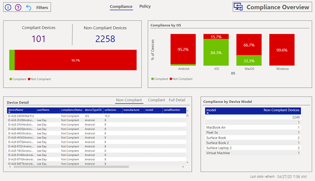
- Compliance Overview

The Compliance Overview page surfaces device compliance data:
- Count of devices in each compliance state
- Counts of devices in each compliance state.
- Compliance by OS
- Vertical bar charts for the percentage of devices in each state by OS.
- Device Detail
- Tabular view of devices, their compliance status and additional information. You can right click on a device record to drill down for even more information on the device. Use the tabs to filter on each status for list of devices.
- Compliance by Device Model
- Counts of number of devices in each compliance state by device model.
The compliance states have been updated to match those in the console. In particular, the status of “Non-compliant” is the sum of “Not compliant” and “In grace period” devices. For more information on the compliance statuses, learn more in the Intune documentation.
You can select a single part of a visualization to set a filter on the rest of the tiles to reflect your selection. The right pane filters can also be used to further slice the data with the available data entities.
2. Policy Overview

The Policy Overview page surfaces the status information for your assigned policies. You can view the data across all your policies or only the top 10 defined by the highest number of assignments.
The policy page shows the following information:
- Policy Adherence % over time
- Chart to show over the percentage of devices with adherence to assigned policies over time. Default time horizon is last 30 days.
- Policy Activity Status over time
- Chart to show the percentage of assigned policy status over time. Default time horizon is last 30 days.
- Current Policy device count
- Tabular view of number of devices assigned to each policy. Select “Full detail” for more information.
Like the Compliance Overview, you can select a record from the table to set a filter across your other charts. Again, use the right pane to further filter and slice the data to your needs.
3. General Information

This page is intended to provide more information around using the compliance report, including frequently asked questions, definitions of terminology used, and links to helpful resources. Here you can navigate to the Intune Data Warehouse and PowerBI documentation, download versions of the PowerBI files and share feedback via UserVoice.
Use the question mark icon on the Compliance Overview and Policy Overview pages to view overlays on the data tiles for extra information.
So how do I download V2?
You can follow the link here to download the new version: https://github.com/microsoft/Intune-Data-Warehouse/tree/master/PowerBIApps
Follow the instructions found here to download the new version: https://docs.microsoft.com/power-bi/service-template-apps-install-distribute#update-a-template-app.
You may see a notification come up in your console prompting you to download V2.
What happens to the old version?
When you are prompted to install the new version, you will see a message like the following:

By default, you will overwrite the current version of the Compliance report with the newer version.
If you wish to maintain access to the previous version, you can download it here: https://github.com/microsoft/Intune-Data-Warehouse/tree/master/PowerBIApps. Note, the information page via the “PBIX file” button will take you to GitHub to access any version you prefer.
Additional Links to getting started with the Intune Data Warehouse and PowerBI
Let us know if you have any additional questions on this by replying back to this post or tagging @IntuneSuppTeam out on Twitter!
by Scott Muniz | Jul 29, 2020 | Alerts, Microsoft, Technology, Uncategorized
This article is contributed. See the original author and article here.
Those responsible for data will tell you that no matter what they do, at the end of the day, they’re value is only seen when the customer can get to the data they want. As much as we want to say this has to do with the data architecture, the design, the platforming and the code, it also has to incorporate the backup, retention and recovery of said data, too.
Oracle on Azure is a less known option for our beloved cloud and for our customers, we spend considerable time on this topic. Again, the data professional is often judged on how good they are by the ability to get the data back in times of crisis. With this in mind, we’re going to talk about backup and recovery for Oracle on Azure, along with key concepts and what to keep in mind when designing and implementing a solution.
Backups Pressure Points
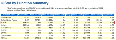
A customer’s RPO and RTO can really impact when going to the cloud. They assume that everything will work the same way as it did on-prem and for most, it really does, but for backups, this is one of the big leaps that have to be made. It’s essential to embrace newer snapshot technologies over older, more archaic utilities for backups and Oracle is no different. We’re already more pressured by IO demands and to add RMAN backups and datapump exports on top of nightly statistics gathering jobs is asking for a perfect storm of IO demands the likes of which no one has ever seen, so this all has to be taken into consideration when architecting the solution.
As we size out the database using extended window AWR reports, we expect backups and any exports to be part of the workload, but if they aren’t, either due to differences in design or products used, this needs to be discussed from the very beginning of the project.

Using all of this information, we are going to identify the VM series not just by the DTU, (combination calculation for CPU and memory) but the VM throughput allowed and then the disk configuration to handle the workload. There are considerable disk options available towards backups, not just blob storage for inexpensive backup dump location, but locally managed disks that can be allocated for faster and more immediate access.
The Discussion
One of the first discussions that should be had when anyone is moving to the cloud around backup and recovery is clearly identifying Recovery Point Objective, (RPO) and Recovery Time Objective, (RTO), which for Oracle, centers around RMAN, Datapump, (imports/exports) and third-party tools.
Recovery Point Objective, (RPO) is the interval of time acceptable before a disruption in the quantity of data lost exceeds the business’ maximum ability to tolerate. Having a clear understanding of what this allowable threshold is essential to determining RPO. Recovery Time Objective (RTO) has to do with how much time it took to recover and return to business. This allowable time duration and any SLA includes when a database must be restored by after an outage or disaster and the time in order to avoid unacceptable consequences associated with a break in business continuity.
Specific questions around expectations for RPO and RTO revolve around:
- What is the time a database will complete a full or incremental backup and how often?
- What time is required to restore to be completed to meet SLAs?
- Are there any dependencies on archive log backups that will impact the first two scenarios?
- Is there the option to restore the entire VM vs. the database level recovery?
- Is it a multi-tier system that more than the database or VM must be considered in the recovery?
When customers use less-modern practices for development and refreshes, it’s important to help them evolve:
- Are there requirements for table level refreshes?
- Is there a subset of table data that can satisfy the request?
- Can objects be exported as needed during the workday?
- Consider snapshot restores
- Once a snapshot is restored to a secondary VM, the datapump copy would be used to retrieve the table to the destination.
- Consider flashback database from a secondary working database that could be used for a remote table copy to the primary database.
- Size considerations for the Flashback Recovery Area, (FRA) must be considered when implementing this solution and archiving must be enabled.
- The idea is flashback copy could be used to take a copy of the table and even use this table to copy over to a secondary database.
- Are database refreshes for secondary environments used for developers and testing?
- Consider using snapshots vs. RMAN clones or full recoveries.
- The latter are both time and resource intensive.
- Snapshots restores to secondary servers can be created in very short turn-around saving considerable time.
These types of changes can make a world of difference for the customers future, allowing them to not just migrate to the cloud, but completely evolve the way they work today.
RMAN on Azure
RMAN, i.e. Recovery Manager, is still our go-to tool for Oracle backups on Azure, but it can add undo pressure on a cloud environment and this has to be recognized as so. Following best practices can help eliminate some of these challenges.
- Ensure that Redo is separated from Data
- Stripe disks and use the correct storage for the IO performance
- Size the VM appropriately, taking VM IO throughput limits into sizing considerations.
- Incorporate optimization features in RMAN, such as parallel matched to number of channels, RATE for throttling backups,
- Compress backup set AFTER and outside of RMAN if time is a consideration
- Turn on optimization:
RMAN> CONFIGURE BACKUP OPTIMIZATION ON;
By default this parameter is set to OFF, which results in Oracle not skipping unchanged data blocks in datafiles or backup of files that haven’t changed. Why backup something that’s already backed up and retained?
If you want to write backups to blob storage, blob fuse will still make a back up to locally managed disk and then move it to the less expensive blob storage. The time taken to perform this copy is what most are concerned about and if the time consideration isn’t a large concern for the customer, we choose to do this, but for those with stricter RPO/RTO, we’re less likely to go this route, choosing locally managed, striped disk instead.
As we’re still dependent on limits per VM on IO throughput, it’s important to take this all into consideration when sizing out the VM series and storage choices. We may size up from an E-series to an M-series that offers higher thresholds and write acceleration, along with ultra disk for our redo logs to assist with archiving. Identifying not only the IO but latency at the Oracle database level is important as these decisions are made. Don’t assume, but gather the information provided in an AWR for when a backup is taken, (datapump or other scenario being researched) to identify the focal point.
For many customers, ensuring that storage best practices around disk striping and mirroring are essential to improve performance of RMAN on Azure IaaS.
Using Azure Site Recovery Snapshots with Oracle
Azure Site Recovery isn’t “Oracle aware” like it is for Azure SQL, SQL Server or other managed database platforms, but that doesn’t mean that you can use it with Oracle. I just assumed that it was evident how to use it with Oracle but discovered that I shouldn’t assume. The key is putting the database in hot backup mode before the snapshot is taken and then taking it back out of backup mode once finished. The snapshot takes a matter of seconds, so it’s a very short amount of time to perform the task and then release the database to proceed forward.
This relies on the following to be performed in a script from a jump box, (not on the database server)
- Main script executes an “az vm run-command invoke” to the Oracle database server and run a script
- Script on the database server receives two arguments: Oracle SID, begin. This places the database into hot backup mode –
alter database begin backup;
- Main script the executes an “az vm snapshot” against each of the drives it captures for the Resource Group and VM Name. Each snapshot only takes a matter of seconds to complete.
- Main script executes an “az vm run-command invoke” to the Oracle database server and run a script
- Script on database server receives two arguments: Oracle SID, end. This takes the database out of hot backup mode
alter database end backup;
- Main script checks log for any errors and if any our found, notifies, if none, exits.
This script would run once per day to take a snapshot that could then be used to recover the VM and the database from.
Third Party Backup Utilities
As much as backup with RMAN is part of the following backup utilities, I’d like to push again for snapshots at the VM level that are also database enforced, allowing for less footprint on the system and quicker recovery times. Note that we again are moving away from full backups in RMAN and moving towards RMAN aware snapshots that can provide us with a database consistent snapshot that can be used to recover from and eliminate extra IO workload on the virtual machine.
Some popular services in the Azure Marketplace that are commonly used by customers for backups and snapshots are:
- Commvault
- Veeam
- Pure Storage Backup
- Rubrik
I’m starting to see a larger variety of tools available that once were only available on-prem. If the customer is comfortable with a specific third-party tool, I’d highly recommend researching and discovering if it’s feasible to also use it in Azure to ease the transition. One of the biggest complaints by customers going to the cloud is the learning curve, so why not make it simpler by keeping those tools that can remain the same, do just that?
by Scott Muniz | Jul 29, 2020 | Alerts, Microsoft, Technology, Uncategorized
This article is contributed. See the original author and article here.
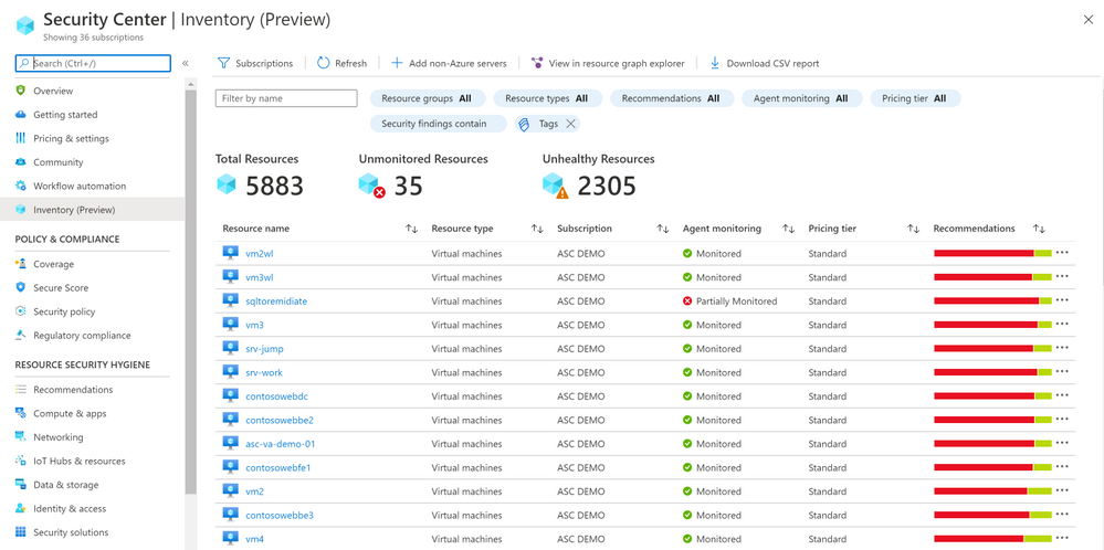
We are delighted to announce that Azure Security Center new Asset Inventory experience is now available in public preview!
What is the Asset Inventory experience?
A novel asset management experience providing you with full visibility over all your Security Center monitored resources.
This enables you to explore your security posture data in a much deeper and meaningful way with enhanced capabilities to filter, export, cross reference with different resource properties in addition to ASC generated insights.
This new experience is fully built on top of Azure Resource Graph (ARG) which now stores all of ASC security posture data, and leveraging its powerful KQL engine enables customers to quickly and easily reach deep insights on top of ASC data and cross reference with any other resource properties.
What can be achieved with this experience?
It is designed to help customers answer questions such as:
What are all my resources that are covered by Azure Security Center and which of these resources have outstanding security recommendations that should get my attention?

Find all resources that are vulnerable by a specific vulnerability and has a specific Azure resource tag?

To view more information about a resource, you can select it. The resource health pane opens.

These are just few examples of what can be discovered in the new experience, both in the UI and programmatically by calling the queries directly from Azure Resource Graph.
To save the query for later use, export it.


You can export the retrieved resources to CSV file for further use.

You can also onboard new Non-Azure servers to Azure Security Center.

As mentioned above, the Asset Inventory experience is now in public preview and will be improved constantly, stay tuned.
by Scott Muniz | Jul 29, 2020 | Alerts, Microsoft, Technology, Uncategorized
This article is contributed. See the original author and article here.
Introduction
Machine Learning is widely used these days for various data driven tasks including detection of security threats, monitoring IoT devices for predictive maintenance, recommendation systems, financial analysis and many other domains. Most ML models are built and deployed in two steps:
- Offline training
- Real time scoring
ML Training is done by researchers/data scientists. They fetch the training data, clean it, engineer features, try different models and tune parameters, repeating this cycle to improve the model’s quality and accuracy. This process is usually done using data science tools such as Jupyter, PyCharm, VS Code, Matlab etc. Once the model meets the required quality it is serialized and saved for scoring.
ML Scoring is the process of applying the model on new data to get insights and predictions. This is actually the business goal for building the model. Scoring usually needs to be done at scale with minimal latency, processing large sets of new records. For ADX users, the best solution for scoring is directly in ADX. ADX scoring is done on its compute nodes, in distributed manner near the data, thus achieving the best performance with minimal latency.
There are many types of models such as Bayesian models, decision trees and forests, regressions, deep neural networks and many more. These models can be built by various frameworks and/or packages like Scikit-learn, Tensorflow, CNTK, Keras, Caffe2, PyTorch etc. (here is a nice overview of ML algorithms, tools and frameworks). On one hand this variety is very good – you can find the most convenient algorithm and framework for your scenario, but on the other hand it creates an interoperability issue, as usually the ML scoring is done on infrastructure which is different from the one used for the training.
To resolve it, Microsoft and Facebook introduced in 2017 ONNX, Open Neural Network Exchange, that was adopted by many companies including AWS, IBM, Intel, Baidu, Mathworks, NVIDIA and many more. ONNX is a system for representation and serialization of ML models to a common file format. This format enables smooth switching among ML frameworks as well as allowing hardware vendors and others to improve the performance of deep neural networks for multiple frameworks at once by targeting the ONNX representation.
In this blog we explain how ADX can consume ONNX models, that were built and trained externally, for near real time scoring of new samples that are ingested into ADX.
How to use ADX for scoring ONNX models
ADX supports running Python code embedded in Kusto Query Language (KQL) using the python() plugin. The Python code is run in multiple sandboxes on ADX existing compute nodes. The Python image is based on Anaconda distribution and contains the most common ML frameworks including Scikit-learn, TensorFlow, Keras and PyTorch. To score ONNX models in ADX follow these steps:
- Develop your ML model using your favorite framework and tools
- Convert the final trained model to ONNX format
- Export the ONNX model to a table on ADX or to an Azure blob
- Score new data in ADX using the inline python() plugin
Example
We build a model to predict room occupancy based on Occupancy Detection data, a public dataset from UCI Repository. This model is a binary classifier to predict occupied/empty room based on Temperature, Humidity, Light and CO2 sensors measurements. The complete process can be found in this Jupyter notebook. Here we embed few snips just to present the main concepts
Prerequisite
- Enable Python plugin on your ADX cluster (see the Onboarding section of the python() plugin doc)
- Whitelist a blob container to be accessible by ADX Python sandbox (see the Appendix section of that doc)
- Create a Python environment (conda or virtual env) that reflects the Python sandbox image
- Install in that environment ONNX packages: onnxruntime and skl2onnx packages
- Install in that environment Azure Blob Storage package: azure-storage-blob
- Install KqlMagic to easily connect and query ADX cluster from Jupyter notebooks
Retrieve and explore the data using KqlMagic
reload_ext Kqlmagic
%config Kqlmagic.auto_dataframe = True
%kql kusto://code;cluster='demo11.westus';database='ML' -try_azcli_login
%kql df << OccupancyDetection
df[-4:]
| |
Timestamp
|
Temperature
|
Humidity
|
Light
|
CO2
|
HumidityRatio
|
Occupancy
|
Test
|
|
20556
|
2015-02-18 09:16:00.0000000
|
20.865
|
27.7450
|
423.50
|
1514.5
|
0.004230
|
True
|
True
|
|
20557
|
2015-02-18 09:16:00.0000000
|
20.890
|
27.7450
|
423.50
|
1521.5
|
0.004237
|
True
|
True
|
|
20558
|
2015-02-18 09:17:00.0000000
|
20.890
|
28.0225
|
418.75
|
1632.0
|
0.004279
|
True
|
True
|
|
20559
|
2015-02-18 09:19:00.0000000
|
21.000
|
28.1000
|
409.00
|
1864.0
|
0.004321
|
True
|
True
|
Train your model
Split the data to features (x), labels (y) and for training/testing:
train_x = df[df['Test'] == False][['Temperature', 'Humidity', 'Light', 'CO2', 'HumidityRatio']]
train_y = df[df['Test'] == False]['Occupancy']
test_x = df[df['Test'] == True][['Temperature', 'Humidity', 'Light', 'CO2', 'HumidityRatio']]
test_y = df[df['Test'] == True]['Occupancy']

print(train_x.shape, train_y.shape, test_x.shape, test_y.shape)
(8143, 5) (8143,) (12417, 5) (12417,)
Train few classic models from Scikit-learn:
from sklearn import tree
from sklearn import neighbors
from sklearn import naive_bayes
from sklearn.linear_model import LogisticRegression
from sklearn.model_selection import cross_val_score

#four classifier types
clf1 = tree.DecisionTreeClassifier()
clf2 = LogisticRegression(solver='liblinear')
clf3 = neighbors.KNeighborsClassifier()
clf4 = naive_bayes.GaussianNB()

clf1 = clf1.fit(train_x, train_y)
clf2 = clf2.fit(train_x, train_y)
clf3 = clf3.fit(train_x, train_y)
clf4 = clf4.fit(train_x, train_y)

# Accuracy on Testing set

for clf, label in zip([clf1, clf2, clf3, clf4], ['Decision Tree', 'Logistic Regression', 'K Nearest Neighbour', 'Naive Bayes']):
            scores = cross_val_score(clf, test_x, test_y, cv=5, scoring='accuracy')
            print("Accuracy: %0.4f (+/- %0.4f) [%s]" % (scores.mean(), scores.std(), label))
Accuracy: 0.8605 (+/- 0.1130) [Decision Tree]
Accuracy: 0.9887 (+/- 0.0071) [Logistic Regression]
Accuracy: 0.9656 (+/- 0.0224) [K Nearest Neighbour]
Accuracy: 0.8893 (+/- 0.1265) [Naive Bayes]
The logistic regression model is the best one
Convert the model to ONNX
from skl2onnx import convert_sklearn
from skl2onnx.common.data_types import FloatTensorType

# We define the input type (5 sensors readings), convert the scikit-learn model to ONNX and serialize it

initial_type = [('float_input', FloatTensorType([None, 5]))]
onnx_model = convert_sklearn(clf2, initial_types=initial_type)
bmodel = onnx_model.SerializeToString()
Test ONNX Model
Predict using ONNX runtime
import numpy as np
import onnxruntime as rt

sess = rt.InferenceSession(bmodel)
input_name = sess.get_inputs()[0].name
label_name = sess.get_outputs()[0].name
pred_onnx = sess.run([label_name], {input_name: test_x.values.astype(np.float32)})[0]

# Verify ONNX and Scikit-learn predictions are same

pred_clf2 = clf2.predict(test_x)
diff_num = (pred_onnx != pred_clf2).sum()

if diff_num:
    print(f'Predictions difference between sklearn and onnxruntime, total {diff_num} elements differ')
else:
    print('Same prediction using sklearn and onnxruntime')
Same prediction using sklearn and onnxruntime
Scoring in ADX
Prerequisite
The Python image of ADX sandbox does NOT include ONNX runtime package. Therefore, we need to zip and upload it to a blob container and dynamically install from that container. Note that the blob container should be whitelisted to be accessible by ADX Python sandbox (see the appendix section of the python() plugin doc)
Here are the steps to create and upload the ONNX runtime package:
- Open Anaconda prompt on your local Python environment
- Download the onnxruntime package, run:
pip wheel onnxruntime
- Zip all the wheel files into onnxruntime-1.4.0-py36.zip (or your preferred name)
- Upload the zip file to a blob in the whitelisted blob container (you can use Azure Storage Explorer)
- Generate a SAS key with read permission to the blob
There are 2 options for retrieving the model for scoring:
- serialize the model to a string to be stored in a standard table in ADX
- copy the model to a blob container (that was previously whitelisted for access by ADX Python sandbox)
Scoring from serialized model which is stored in ADX table
Serializing the model and store it in ADX models table using KqlMagic
import pandas as pd
import datetime

models_tbl = 'ML_Models'
model_name = 'ONNX-Occupancy'

smodel = bmodel.hex()
now = datetime.datetime.now()
dfm = pd.DataFrame({'name':[model_name], 'timestamp':[now], 'model':[smodel]})
dfm
| |
name
|
timestamp
|
model
|
|
0
|
ONNX-Occupancy
|
2020-07-28 17:07:20.280040
|
08031208736b6c326f6e6e781a05312e362e3122076169…
|
set_query = '''
.set-or-append {0} <|
let tbl = dfm;
tbl
'''.format(models_tbl)
print(set_query)
.set-or-append ML_Models <|
let tbl = dfm;
tbl
%kql -query set_query
| |
ExtentId
|
OriginalSize
|
ExtentSize
|
CompressedSize
|
IndexSize
|
RowCount
|
|
0
|
bfc9acc2-3d79-4e64-9a79-d2681547e43d
|
1430.0
|
1490.0
|
1040.0
|
450.0
|
1
|
Scoring from serialized model which is stored in ADX table
# NOTE: we run ADX scoring query here using KqlMagic by embedding the query from Kusto Explorer
# with r'''Kusto Explorer query''':

# NOTE: replace the string "**** YOUR SAS KEY ****" in the external_artifacts parameter with the real SAS

scoring_from_table_query = r'''
let classify_sf=(samples:(*), models_tbl:(name:string, timestamp:datetime, model:string), model_name:string, features_cols:dynamic, pred_col:string)
{
    let model_str = toscalar(models_tbl | where name == model_name | top 1 by timestamp desc | project model);
    let kwargs = pack('smodel', model_str, 'features_cols', features_cols, 'pred_col', pred_col);
    let code =
    'n'
    'import picklen'
    'import binasciin'
    'n'
    'smodel = kargs["smodel"]n'
    'features_cols = kargs["features_cols"]n'
    'pred_col = kargs["pred_col"]n'
    'bmodel = binascii.unhexlify(smodel)n'
    'n'
    'from sandbox_utils import Zipackagen'
    'Zipackage.install("onnxruntime-v17-py36.zip")n'
    'features_cols = kargs["features_cols"]n'
    'pred_col = kargs["pred_col"]n'
    'n'
    'import onnxruntime as rtn'
    'sess = rt.InferenceSession(bmodel)n'
    'input_name = sess.get_inputs()[0].namen'
    'label_name = sess.get_outputs()[0].namen'
    'df1 = df[features_cols]n'
    'predictions = sess.run([label_name], {input_name: df1.values.astype(np.float32)})[0]n'
    'n'
    'result = dfn'
    'result[pred_col] = pd.DataFrame(predictions, columns=[pred_col])'
    'n'
    ;
    samples | evaluate python(typeof(*), code, kwargs, external_artifacts=pack('onnxruntime-v17-py36.zip', 'https://artifcatswestus.blob.core.windows.net/kusto/ONNX/onnxruntime-v17-py36.zip? **** YOUR SAS KEY ****')
)
};
OccupancyDetection
| where Test == 1
| extend pred_Occupancy=bool(0)
| invoke classify_sf(ML_Models, 'ONNX-Occupancy', pack_array('Temperature', 'Humidity', 'Light', 'CO2', 'HumidityRatio'), 'pred_Occupancy')
'''

%kql pred_df << -query scoring_from_table_query

pred_df[-4:]
| |
Timestamp
|
Temperature
|
Humidity
|
Light
|
CO2
|
HumidityRatio
|
Occupancy
|
Test
|
pred_Occupancy
|
|
12413
|
2015-02-18 09:16:00+00:00
|
20.865
|
27.7450
|
423.50
|
1514.5
|
0.004230
|
True
|
True
|
True
|
|
12414
|
2015-02-18 09:16:00+00:00
|
20.890
|
27.7450
|
423.50
|
1521.5
|
0.004237
|
True
|
True
|
True
|
|
12415
|
2015-02-18 09:17:00+00:00
|
20.890
|
28.0225
|
418.75
|
1632.0
|
0.004279
|
True
|
True
|
True
|
|
12416
|
2015-02-18 09:19:00+00:00
|
21.000
|
28.1000
|
409.00
|
1864.0
|
0.004321
|
True
|
True
|
True
|
print('Confusion Matrix')
pred_df.groupby(['Occupancy', 'pred_Occupancy']).size()
Confusion Matrix
Occupancy pred_Occupancy
False False 9284
True 112
True False 15
True 3006
Scoring from model which is stored in blob storage
Copy the model to blob
Note again that the blob container should be whitelisted to be accessible by ADX Python sandbox
from azure.storage.blob import BlobClient

conn_str = "BlobEndpoint=https://artifcatswestus.blob.core.windows.net/kusto;SharedAccessSignature=?**** YOUR SAS KEY ****"
blob_client = BlobClient.from_connection_string(conn_str, container_name="ONNX", blob_name="room_occupancy.onnx")

res = blob_client.upload_blob(bmodel, overwrite=True)
# NOTE: we run ADX scoring query here using KqlMagic by embedding the query from Kusto Explorer
# with r'''Kusto Explorer query''':

# NOTE: replace the strings "**** YOUR SAS KEY ****" below with the respective real SAS

scoring_from_blob_query = r'''
let classify_sf=(samples:(*), model_sas:string, features_cols:dynamic, pred_col:string)
{
    let kwargs = pack('features_cols', features_cols, 'pred_col', pred_col);
    let code =
    'n'
    'from sandbox_utils import Zipackagen'
    'Zipackage.install("onnxruntime-v17-py36.zip")n'
    'features_cols = kargs["features_cols"]n'
    'pred_col = kargs["pred_col"]n'
    'n'
    'import onnxruntime as rtn'
    'sess = rt.InferenceSession(r"C:Tempmodel.onnx")n'
    'input_name = sess.get_inputs()[0].namen'
    'label_name = sess.get_outputs()[0].namen'
    'df1 = df[features_cols]n'
    'predictions = sess.run([label_name], {input_name: df1.values.astype(np.float32)})[0]n'
    'n'
    'result = dfn'
    'result[pred_col] = pd.DataFrame(predictions, columns=[pred_col])'
    'n'
    ;
    samples | evaluate python(typeof(*), code, kwargs,
        external_artifacts=pack('model.onnx', model_sas,
                                'onnxruntime-v17-py36.zip', 'https://artifcatswestus.blob.core.windows.net/kusto/ONNX/onnxruntime-v17-py36.zip? **** YOUR SAS KEY ****')
)
};
OccupancyDetection
| where Test == 1
| extend pred_Occupancy=bool(0)
| invoke classify_sf('https://artifcatswestus.blob.core.windows.net/kusto/ONNX/room_occupancy.onnx? **** YOUR SAS KEY ****',
                     pack_array('Temperature', 'Humidity', 'Light', 'CO2', 'HumidityRatio'), 'pred_Occupancy')
'''

%kql pred_df << -query scoring_from_blob_query
pred_df[-4:]
| |
Timestamp
|
Temperature
|
Humidity
|
Light
|
CO2
|
HumidityRatio
|
Occupancy
|
Test
|
pred_Occupancy
|
|
12413
|
2015-02-18 09:16:00+00:00
|
20.865
|
27.7450
|
423.50
|
1514.5
|
0.004230
|
True
|
True
|
True
|
|
12414
|
2015-02-18 09:16:00+00:00
|
20.890
|
27.7450
|
423.50
|
1521.5
|
0.004237
|
True
|
True
|
True
|
|
12415
|
2015-02-18 09:17:00+00:00
|
20.890
|
28.0225
|
418.75
|
1632.0
|
0.004279
|
True
|
True
|
True
|
|
12416
|
2015-02-18 09:19:00+00:00
|
21.000
|
28.1000
|
409.00
|
1864.0
|
0.004321
|
True
|
True
|
True
|
print('Confusion Matrix')
pred_df.groupby(['Occupancy', 'pred_Occupancy']).size()
Confusion Matrix
Occupancy pred_Occupancy
False False 9284
True 112
True False 15
True 3006
Summary
In this tutorial we showed how to train a model in Scikit-learn, convert it to ONNX format and export it to ADX for scoring. This workflow is convenient as
- Training can be done on any hardware platform, using any framework supporting ONNX
- Scoring is done in ADX near the data, on the existing compute nodes, enabling near real time processing of big amounts of new data. There is no the need to export the data to external scoring service and import back the results. Consequently, scoring architecture is simpler and performance is much faster and scalable
by Scott Muniz | Jul 29, 2020 | Uncategorized
This article is contributed. See the original author and article here.
Abstract
With the Azure Machine Learning service, the training and scoring of hundreds of thousands of models with large amounts of data can be completed efficiently leveraging pipelines where certain steps like model training and model scoring run in parallel on large scale out compute clusters. In order to help organizations get a head start on building such pipelines, the Many Models Solution Accelerator has been created. The Many Models Solution Accelerator provides two primary examples, one using custom machine learning and the other using AutoML. Give it a try today!
Executive Overview
Many executives are looking to Machine Learning to improve their business. With the reliance on a more digital world, the amount of data generated is increasing faster than ever. Further, companies are purchasing 3rd party datasets to combine with internal data to gain further insight and make better predictions. In order to make better predictions, sophisticated machine learning models are being built that leverages this large pool of data. Further, as companies are expanding to do business in a variety of markets and environments, general machine learning model no longer suffice, instead, more specific machine learning models are needed. In this case, “general machine learning models” refers to the granularity for which this model was built, for example, building a demand forecast model for a product at the country level versus at the city level which would be a “specific machine learning model.” Building more specific machine learning models can easily results in building hundreds of thousands of specific models instead of a handful of general models. Combining large datasets with the need of building hundreds of thousands of more specific machine learning models is not a trivial task. Doing so requires very large compute power. In fact, this task can greatly benefit from parallel compute power where multiple compute instances are working simultaneously to build the machine learning models in parallel. Once those models are trained, leveraging them to score large amounts of data presents the same problem characteristics which again, leveraging a compute cluster where multiple compute instances are making predictions using the machine learning models simultaneously can greatly reduce the time required to do so. With the Azure Machine Learning service, the training and scoring of hundreds of thousands of models with large amounts of data can be completed efficiently leveraging pipelines where certain steps like model training and model scoring run in parallel on large scale out compute clusters. In order to help organizations get a head start on building such pipelines, the Many Models Solution Accelerator has been created. The Many Models Solution Accelerator provides two primary examples, one using custom machine learning and the other using AutoML.
In Azure Machine Learning, AutoML automates the building of the most common categories of Machine Learning models in a very robust and sophisticated manner. For example, a very common machine learning problem is demand forecasting. Having a more accurate demand forecast can increase revenues and reduce waste. Traditionally, many statistical methods have been used to do just this. However, more modern techniques leverage Machine Learning including Deep Learning techniques to provide a more accurate demand forecast. Further, the demand forecast can be improved by moving from forecasting a broader scope (general machine learning model) to forecasting a more granular scope (specific machine learning model). Doing so means, for example, instead of building one forecast for each Product at the country level, building a forecast for each product at the city. Moving to more specific models results in building hundreds of thousands of forecasts using large amounts of data which as discussed above can be solved using the Many Models Solution Accelerator.
Technical Overview
As data scientist move from building a handful of general machine learning models to hundreds of thousands of more specific machine learning models (i.e. geography or product scope), the need to perform the model training and model scoring tasks require parallel compute power to finish in a timely manner. In the Azure Machine Learning service SDK, this is accomplished using Pipelines and specifically a ParallelRunStep which runs on a multi node Compute Clusters. The data scientist provides the ParallelRunStep a custom script, an input dataset, a compute cluster and the amount of parallelism they would like. This concept can be applied to a custom python script and to Automated Machine Learning (AutoML).
Automated Machine Learning (AutoML) uses over ten algorithms (including deep learning algorithms) with varying hyperparameters to build Classification, Regression and Forecasting models. Further, Pipelines automate the invocation of AutoML across multiple nodes using ParallelRunStep to train the models in parallel as well as to batch score new data. Pipelines can be scheduled to run within Azure Machine Learning or invoked using their REST endpoint from various Azure services (i.e. Azure Data Factory, Azure DevOps, Azure Functions, Azure Logic Apps, etc). When invoked, the Parallel Pipelines run on Compute Clusters within Azure Machine Learning. The Compute clusters can be scaled up and out to perform the training and scoring. Each node in a compute clusters can be have Terabytes of RAM, over a 100 cores, and multiple GPUs. Finally, the scored data can be stored in an a datastore in Azure, such as Azure DataLake Gen 2, and then copied to a specific location for an application to consume the results.
In order to provide a jump start in leveraging Pipelines with the new ParallelRunStep, the Many Models Solution Accelerator has been created. This solution accelerator showcases both a custom python script and an AutoML script.
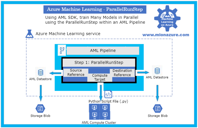
Major Components
The main components of the Many Models Solution Accelerator includes an Azure Machine Learning Workspace, a Pipeline, a ParallelRunStep, a Compute Target, a Datastore, and a Python Script File as depicted in Figure 1, below.

Figure 1. The architecture of a Pipeline with a ParallelRunStep
For an overview of getting started with Azure Machine Learning service, please see the blog article MLonAzure: Getting Started with Azure Machine Learning service for the Data Scientist
For an overview of Pipelines, please see blog article, MLonAzure: Azure Machine Learning service Pipelines
Major Steps
1. Prerequisites
2. Data Prep
- Data needs to be split into multiple files (.csv or .parquet) for each group that a model is to be created for. Each file must contain one or more entire time series for the give group.
- The data must be placed in Azure Storage (e.g. ADL Gen 2, Blob Storage). The storage will then be registered as a Datastore from which two FileDatasets will be registered, one pointing to the folder containing the training data and the other to the folder containing the data to be scored.
- For example, to build a forecast model for each brand within a store, the training sales data would be split to create files StoreXXXX_BrandXXXX.
3. Model Training
The solution accelerator showcases model training with a custom python script and with AutoML which are orchestrated using a Pipeline. Please see solution-accelerator-manymodels-customscript and solution-accelerator-manymodels-AutoML. Putting it all together results in the architecture depicted in Figure 2, below.

Figure 2: Solution Accelerator Model Training
3. a. Pipeline
The solution accelerator leverages the Pipeline object to train the model. Specifically, a ParallelRunStep is used which requires a configuration parameters, ParallelRunConfig
ParallelRunConfig has many parameters, below are the typical ones used for the Many Models Solution Accelerator. For a complete list of ParallelRunConfig parameters, please see the ParallelRunConfig Class.
|
Parameter
|
Explanation
|
|
environment
|
Provides the configurations for the Python Environment
|
|
Entry_script
|
This is a Python file (.py extension only) that will run in parallel. Note that the Many Models Solution Accelerator contains a custom Entry_script that leverages AutoML and one that leverages custom code.
|
|
Compute_target
|
The AML ComputeCluster to run the step on.
|
|
Node_count
|
The number of nodes to use within the training cluster. Scale this number to a higher number to increase parallelism.
|
|
Process_count_per_node
|
The number of cores that will be used within each node
|
|
mini_batch_size
|
For FileDatasets it’s the number of files that are used at a time, for Tabular Datasets it’s the number data size that will be processed at a given time.
|
|
Run_inovcation_timeout
|
The overall allowed time for the parallel run step
|
3. b. Training script with AutoML
The solution accelerator showcases using AutoML Forecasting. AutoML has many parameters, below are the typical ones used for doing a Forecasting task within the Many Models Solution Accelerator. For a complete list of AutoML Config parameters, please see the AutoMLConfig Class.
automl_settings = {
    "task" : 'forecasting',
    "primary_metric" : 'normalized_root_mean_squared_error',
    "iteration_timeout_minutes" : 10,
    "iterations" : 15,
    "experiment_timeout_hours" : 1,
    "label_column_name" : 'Quantity',
    "n_cross_validations" : 3,
    "verbosity" : logging.INFO,
    "debug_log": 'DebugFileName.txt',
    "time_column_name": 'WeekStarting',
    "max_horizon" : 6,
    "group_column_names": ['Store', 'Brand'],
    "grain_column_names": ['Store', 'Brand']
}
|
Parameter
|
Explanation
|
|
task
|
The type of AutoML Task: Classification, Regression, Forecasting
|
|
primary_metric
|
The metric that AutoML should optimize based on
|
|
Iteration_timeout_minutes
|
How long each of the number of “iterations” can run for
|
|
Iterations
|
Number of models that should be tried (combinations of various Algorithms + various Hyperparameters)
|
|
Experiment_timeout_hours
|
How long the overall AutoML Experiment can take. Note: The experiment may might timeout before all iterations are complete.
|
|
label_column_name
|
The column that is being predicted
|
|
n_cross_validations
|
Number of cross validations that should take place within the training dataset
|
|
verbosity
|
Log details
|
|
debug_log
|
Location for the debug log
|
|
time_column_name
|
The name of the Time column, note that the training dataset can have multiple time series
|
|
max_horizon
|
How far how the forecast will go
|
|
group_column_names
|
The names of columns used to group your models. For timeseries, the groups must not split up individual time-series. That is, each group must contain one or more whole time-series.
|
|
grain_column_names
|
The column names used to uniquely identify timeseries in data that has multiple rows with the same timestamp.
|
4. Model Forecasting
The solution accelerator showcases model forecasting with a custom python script and with AutoML which are orchestrated using a Pipeline. Please see solution-accelerator-manymodels-customscript and solution-accelerator-manymodels-AutoML. Putting it all together results in the architecture depicted in Figure 3, below.

Figure 3: Solution Accelerator Model Scoring
5. Automation
In order to automate the solution, the training and scoring pipelines must be published and a PipelineEndPoint must be created. Once that’s done, the PipelineEndpoint can then be invoked from Azure Data Factory. Specifically, the Azure Machine Learning Pipeline Activity is used. Note that the training and scoring pipelines can be collapsed into one pipelines if the training and scoring occur consecutively.
Next Steps
Azure Machine Learning Documentation
Many Models Solution Accelerator
Many Models Solution Accelerator Video
Azure Data Factory: Azure Machine Learning Pipeline Activity
MLOnAzure GitHub: Getting started with Pipelines
MLonAzure Blog: Getting Started with Azure Machine Learning for the Data Scientist
MLonAzure Blog: Azure Machine Learning service Pipelines

Recent Comments