by Contributed | Jul 19, 2021 | Technology
This article is contributed. See the original author and article here.
The use case is as follows: I have water meter telemetry I would like to do analytics on.
Events are ingested from water meters and collected into a data lake in parquet format. The data is partitioned by Year, Month and Day based on the timestamp contained in the events themselves and not based on the time of the event processing in ASA as this is a frequent requirement.
Events are sent from the on premise SCADA systems to Event Hub then processed by Stream Analytics which then can easily:
- Convert events sent in JSON format into partitioned parquet.
- Portioning is based on Year/Month/Day.
- Date used for partitioning is coming from within the event.
The result can immediately be queried with serverless Synapse SQL pool.
Input Stream
My ASA input stream named inputEventHub is plugged into an Event Hub in JSON format.
Output Stream
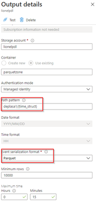
The output stream is the interesting part and will define the partition scheme:
We see that its path pattern is based on a pseudo column named “time_struct” and all the partitioning logic is in the construct of this pseudo column.
Let’s have a look at the ASA query:


We can see now that the pseudo_column time_struct contains the path, ASA understands it and processes it literally including the “/” sign.
Here is the query code:
select
    concat('year=',substring(createdAt,1,4),'/month=',substring(createdAt,6,2),'/day=',substring(createdAt,9,2)) as time_struct,
    eventId,
    [type],
    deviceId,
    deviceSequenceNumber,
    createdAt,
    Value,
    complexData,
    EventEnqueuedUtcTime AS enqueuedAt,
    EventProcessedUtcTime AS processedAt,
    cast(UDF.GetCurrentDateTime('') as datetime) AS storedAt,
    PartitionId
into
    [lionelpdl]
from
    [inputEventHub]
After few days of processing the output folder looks like this as a result:


Query results with serveless SQL and take advantage of partitioning
Now I can directly query my Output Stream with serverless SQL:

We can also notice that the metadata functions are fully functional without any additional work. For example I can run the following query using filepath metadata function:
  SELECT top 100
    [result].filepath(1) AS [year]
    ,[result].filepath(2) AS [month]
    ,[result].filepath(3) AS [day]
    ,*
FROM
    OPENROWSET(
        BULK 'https://lionelpdl.dfs.core.windows.net/parquetzone/deplasa1/year=*/month=*/day=*/*.parquet',
        FORMAT='PARQUET'
    ) AS [result]

where [result].filepath(2)=6
  and [result].filepath(3)=23
Spark post processing
Finally, to optimize my query performance I can schedule a Spark job which processes daily all events from the previous day, compacts them into fewer and larger parquet files.
As an example, I’ve decided to rebuild the partitions with files containing 2 million rows.
Here are 2 versions of the same code:
PySpark notebook (for interactive testing for instance)
from pyspark.sql import SparkSession
from pyspark.sql.types import *
from functools import reduce
from pyspark.sql import DataFrame
import datetime

account_name = "storage_account_name"
container_name = "container_name"
source_root = "source_directory_name"
target_root = "target_directory_name"
days_backwards = 4 #number of days from today, typicaly, as a daily job it'll be set to 1
adls_path = 'abfss://%s@%s.dfs.core.windows.net/%s' % (container_name, account_name, source_root)

hier = datetime.date.today() - datetime.timedelta(days = days_backwards)
day_to_process = '/year=%04d/month=%02d/day=%02d/' % (hier.year,hier.month,hier.day)
file_pattern='*.parquet'

print((adls_path + day_to_process + file_pattern))

df = spark.read.parquet(adls_path + day_to_process + file_pattern)

adls_result = 'abfss://%s@%s.dfs.core.windows.net/%s' % (container_name, account_name, target_root)

print(adls_result + day_to_process + file_pattern)

df.coalesce(1).write.option("header",True)
        .mode("overwrite")
        .option("maxRecordsPerFile", 2000000)
        .parquet(adls_result + day_to_process)
Spark job (with input parameters scheduled daily)

import sys
import datetime
from pyspark import SparkContext, SparkConf
from pyspark.sql import SparkSession
from pyspark.sql.types import *
from functools import reduce
from pyspark.sql import DataFrame

if __name__ == "__main__":

	# create Spark context with necessary configuration
	conf = SparkConf().setAppName("dailyconversion").set("spark.hadoop.validateOutputSpecs", "false")
	sc = SparkContext(conf=conf)
	spark = SparkSession(sc)

	account_name = sys.argv[1] #'storage_account_name'
	container_name = sys.argv[2] #"container_name"
	source_root = sys.argv[3] #"source_directory_name"
	target_root = sys.argv[4] #"target_directory_name"
	days_backwards = sys.argv[5] #number of days backwards in order to reprocess the parquet files, typically 1

	hier = datetime.date.today() - datetime.timedelta(days=int(days_backwards))

	day_to_process = '/year=%04d/month=%02d/day=%02d/' % (hier.year,hier.month,hier.day)
	file_pattern='*.parquet'

	adls_path = 'abfss://%s@%s.dfs.core.windows.net/%s' % (container_name, account_name, source_root)

	print((adls_path + day_to_process + file_pattern))

	df = spark.read.parquet(adls_path + day_to_process + file_pattern)
	#display (df.limit(10))
	#df.printSchema()
	#display(df)
	adls_result = 'abfss://%s@%s.dfs.core.windows.net/%s' % (container_name, account_name, target_root)

	print(adls_result + day_to_process + file_pattern)

	df.coalesce(1).write.option("header",True)
		.mode("overwrite")
		.option("maxRecordsPerFile", 2000000)
		.parquet(adls_result + day_to_process)
Conclusion
In this article we have covered:
- How to easily use Stream Analytics to write an output with partitioned parquet files.
- How to use serverless Synapse SQL pool to query Stream analytics output.
- How to reduce the number of parquet files using synapse Spark pool.
Additional resources:
by Contributed | Jul 17, 2021 | Technology
This article is contributed. See the original author and article here.
By Evan Rust and Zin Thein Kyaw
Introduction
Wheel lug nuts are such a tiny part of the overall automobile assembly that they’re easy to overlook, but yet serve a critical function in the safe operation of an automobile. In fact, it is not safe to drive even with one lug nut missing. A single missing lug nut will cause increased pressure on the wheel, in turn causing damage to the wheel bearings, studs, and make the other lug nuts fall off.
Over the years there have been a number of documented safety recalls and issues around wheel lug nuts. In some cases, it was only identified after the fact that the automobile manufacturer had installed incompatible lug nut types with the wheel or had been inconsistent in installing the right type of lug nut. Even after delivery, after years of wear and tear, the lug nuts may become loose and may even fall off which would cause instability for an automobile to be in service. To reduce these incidents of quality control at manufacturing and maintenance in the field, there is a huge opportunity to leverage machine learning at the edge to automate wheel lug nut detection.
This motivated us to create a proof-of-concept reference project for automating wheel lug nut detection by easily putting together a USB webcam, Raspberry Pi 4, Microsoft Azure IoT, and Edge Impulse, creating an end-to-end wheel lug nut detection system using Object Detection. This example use case and other derivatives will find a home in many industrial IoT scenarios where embedded Machine Learning can help improve the efficiency of factory automation and quality control processes including predictive maintenance.
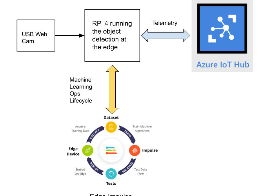
This reference project will serve as a guide for quickly getting started with Edge Impulse on the Raspberry Pi 4 and Azure IoT, to train a model that detects lug nuts on a wheel and sends inference conclusions to Azure IoT as shown in the block diagram below:

Design Concept: Edge Impulse and Azure IoT
Edge Impulse is an embedded machine learning platform that allows you to manage the entire Machine Learning Ops (MLOps) lifecycle which includes 1) Data Acquisition, 2) Signal Processing, 3) ML Training, 4) Model Testing, and 5) Creating a deployable model that can run efficiently on an edge device.
For the edge device, we chose to use the Raspberry Pi 4 due to its ubiquity and available processing power for efficiently running more sophisticated machine learning models such as object detection. By running the object detection model on the Raspberry Pi 4, we can optimize the network bandwidth connection to Azure IoT for robustness and scalability by only sending the inference conclusions, i.e. “How many lug nuts are on the wheel?”. Once the inference conclusions are available at the Azure IoT level, it becomes straightforward to feed these results into your business applications that can leverage other Azure services such as Azure Stream Analytics and Power BI.
In the next sections we’ll discuss how you can set this up yourself with the following items:
Setting Up the Hardware
We begin by setting up the Raspberry Pi 4 to connect to a Wi-Fi network for our network connection, configuring it for camera support, and installing the Edge Impulse Linux CLI (command line interface) tools on the Raspberry Pi 4. This will allow the Raspberry Pi 4 to directly connect to Edge Impulse for data acquisition and finally, deployment of the wheel lug nut detection model.

For starters, you’ll need a Raspberry Pi 4 with an up-to-date Raspberry Pi OS image that can be found here. After flashing this image to an SD card and adding a file named ‘wpa_supplicant.conf’:
ctrl_interface=DIR=/var/run/wpa_supplicant GROUP=netdev
update_config=1
country=<Insert 2 letter ISO 3166-1 country code here>
network={
 ssid="<Name of your wireless LAN>"
 psk="<Password for your wireless LAN>"
}
along with an empty file named ‘ssh’ (both within the ‘/boot’ directory), you can go ahead and power up the board.
Once you’ve successfully SSH’d into the device with
ssh pi@<IP_ADDRESS>
and the password ‘raspberry’, it’s time to install the dependencies for the Edge Impulse Linux SDK. Simply run the next three commands to set up the NodeJS environment and everything else that’s required for the edge-impulse-linux wizard:
curl -sL https://deb.nodesource.com/setup_12.x | sudo bash -
sudo apt install -y gcc g++ make build-essential nodejs sox gstreamer1.0-tools gstreamer1.0-plugins-good gstreamer1.0-plugins-base gstreamer1.0-plugins-base-apps
npm config set user root && sudo npm install edge-impulse-linux -g --unsafe-perm
For more details on setting up the Raspberry Pi 4 with Edge Impulse, visit this link.
Since this project deals with images, we’ll need some way to capture them. The wizard supports both the Pi camera modules and standard USB webcams, so make sure to enable the camera module first with
sudo raspi-config
if you plan on using one. With that completed, go to Edge Impulse and create a new project, then run the wizard with
edge-impulse-linux
and make sure your device appears within the Edge Impulse Studio’s device section after logging in and selecting your project.

Data Acquisition
Training accurate production ready machine learning models requires feeding plenty of varied data, which means a lot of images are typically required. For this proof-of-concept, we captured around 145 images of a wheel that had lug nuts on it. The Edge Impulse Linux daemon allows you to directly connect the Raspberry Pi 4 to Edge Impulse and take snapshots using the USB webcam.

Using the Labeling queue in the Data Acquisition page we then easily drew bounding boxes around each lug nut within every image, along with every wheel. To add some test data we went back to the main Dashboard page and clicked the ‘Rebalance dataset’ button that moves 20% of the training data to the test data bin.
Impulse Design and Model Training
Now that we have plenty of training data, it’s time to design and build our model. The first block in the Impulse Design is an Image Data block, and it scales each image to a size of ‘320’ by ‘320’ pixels.

Next, image data is fed to the Image processing block that takes the raw RGB data and derives features from it.

Finally, these features are used as inputs to the MobileNetV2 SSD FPN-Lite Transfer Learning Object Detection model that learns to recognize the lug nuts. The model is set to train for ’25’ cycles at a learning rate of ‘.15’, but this can be adjusted to fine-tune for accuracy. As you can see from the screenshot below, the trained model indicates a precision score of 97.9%.

Model Testing
If you’ll recall from an earlier step we rebalanced the dataset to put 20% of the images we collected to be used for gauging how our trained model could perform in the real world. We use the model testing page to run a batch classification and see how we expect our model to perform. The ‘Live Classification’ tab will also allow you to acquire new data direct from the Raspberry Pi 4 and see how the model measures up against the immediate image sample.

Versioning
An MLOps platform would not be complete without a way to archive your work as you iterate on your project. The ‘Versioning’ tab allows you to save your entire project including the entire dataset so you can always go back to a “known good version” as you experiment with different neural network parameters and project configurations. It’s also a great way to share your efforts as you can designate any version as ‘public’ and other Edge Impulse users can clone your entire project and use it as a springboard to add their own enhancements.

Deploying Models
In order to verify that the model works correctly in the real world, we’ll need to deploy it to the Raspberry Pi 4. This is a simple task thanks to the Edge Impulse CLI, as all we have to do is run
edge-impulse-linux-runner
which downloads the model and creates a local webserver. From here, we can open a browser tab and visit the address listed after we run the command to see a live camera feed and any objects that are currently detected. Here’s a sample of what the user will see in their browser tab:

Sending Inference Results to Azure IoT Hub
With the model working locally on the Raspberry Pi 4, let’s see how we can send the inference results from the Raspberry Pi 4 to an Azure IoT Hub instance. As previously mentioned, these results will enable business applications to leverage other Azure services such as Azure Stream Analytics and Power BI. On your development machine, make sure you’ve installed the Azure CLI and have signed in using ‘az login’. Then get the name of the resource group you’ll be using for the project. If you don’t have one, you can follow this guide on how to create a new resource group.

After that, return to the terminal and run the following commands to create a new IoT Hub and register a new device ID:
az iot hub create --resource-group <your resource group> --name <your IoT Hub name>
az extension add --name azure-iot
az iot hub device-identity create --hub-name <your IoT Hub name> --device-id <your device id>

Retrieve the connection string the Raspberry Pi 4 will use to connect to Azure IoT with:
az iot hub device-identity connection-string show --device-id <your device id> --hub-name <your IoT Hub name>

Now it’s time to SSH into the Raspberry Pi 4 and set the connection string as an environment variable with:
export IOTHUB_DEVICE_CONNECTION_STRING="<your connection string here>"
Then, add the necessary Azure IoT device libraries with:
pip install azure-iot-device
(Note: if you do not set the environment variable or pass it in as an argument the program will not work!) The connection string contains the information required for the Raspberry Pi 4 to establish a connection with the Azure IoT Hub service and communicate with it. You can then monitor output in the Azure IoT Hub with:
az iot hub monitor-events --hub-name <your IoT Hub name> --output table
or in the Azure Portal.

To make sure it works, download and run this example on the Raspberry Pi 4 to make sure you can see the test message.
For the second half of deployment, we’ll need a way to customize how our model is used within the code. Edge Impulse provides a Python SDK for this purpose. On the Raspberry Pi 4 install it with
sudo apt-get install libatlas-base-dev libportaudio0 libportaudio2 libportaudiocpp0 portaudio19-dev
pip3 install edge_impulse_linux -i https://pypi.python.org/simple
We’ve made available a simple example on the Raspberry Pi 4 that sets up a connection to the Azure IoT Hub, runs the model, and sends the inference results to Azure IoT.

Once you’ve either downloaded the zip file or cloned the repo into a folder, get the model file by running
edge-impulse-linux-runner --download modelfile.eim
inside of the folder you just created from the cloning process. This will download a file called ‘modelfile.eim’. Now, run the Python program with
python lug_nut_counter.py ./modelfile.eim -c <LUG_NUT_COUNT>
where <LUG_NUT_COUNT> is the correct number of lug nuts that should be attached to the wheel (you might have to use ‘python3’ if both Python 2 and 3 are installed).

Now whenever a wheel is detected the number of lug nuts is calculated. If this number falls short of the target, a message is sent to the Azure IoT Hub.

And by only sending messages when there’s something wrong, we can prevent an excess amount of bandwidth from being taken due to empty payloads.

Conclusion
We’ve just scratched the surface with wheel lug nut detection. Imagine utilizing object detection for other industrial applications in quality control, detecting ripe fruit amongst rows of crops, or identifying when machinery has malfunctioned with devices powered by machine learning.
With any hardware, Edge Impulse, and Microsoft Azure IoT, you can design comprehensive embedded machine learning models, deploy them on any device, while authenticating each and every device with built-in security. You can set up individual identities and credentials for each of your connected devices to help retain the confidentiality of both cloud-to-device and device-to-cloud messages, revoke access rights for specific devices, upgrade device firmware remotely, and benefit from advanced analytics on devices running offline or with intermittent connectivity.
The complete Edge Impulse project is available here for you to see how easy it is to start building your own embedded machine learning projects today using object detection. We look forward to your feedback at hello@edgeimpulse.com or on our forum.


Recent Comments