Improving Postgres Connection Scalability: Snapshots

Improving Postgres Connection Scalability: Snapshots

This article is contributed. See the original author and article here.

I recently analyzed the limits of connection scalability, to understand the most effective way to improve Postgres’ handling of large numbers of connections, and why that is important. I concluded that the most pressing issue is snapshot scalability.


This post details the improvements I recently contributed to Postgres 14 (to be released Q3 of 2021), significantly reducing the identified snapshot scalability bottleneck.


pgbench-before-and-after-performance-comparison-Postgres-snapshot-scalability-v2-1920x1080.jpg


As the explanation of the implementation details is fairly long, I thought it’d be more fun for of you if I start with the results of the work, instead of the technical details (I’m cheating, I know ;)).


First: Performance Improvements


For all of these benchmarks, I compared the Postgres development tree just before and after all the connection scalability changes have been merged. There are a few other changes interspersed, but none that are likely to affect performance in a significant way.


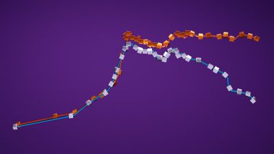
First, a before / after comparison of a read-only pgbench benchmark, on an Azure F72s_v2 VM:


Figure 1: Benchmark (read-only pgbench) results comparison, showing the effects of the snapshot scalability improvements.Figure 1: Benchmark (read-only pgbench) results comparison, showing the effects of the snapshot scalability improvements.


These results 1 show a significant improvement after the snapshot scalability changes I’ll be talking about in this post, with little evidence of scalability issues even at very high connection counts. The dip starting around 100 connections—for both the pre/post changes runs— appears to be caused by OS task scheduling, rather than Postgres directly.


Next up, a repeat of the benchmarks I used in my last post on analyzing connection scalability to identify snapshot scalability as the primary bottleneck (again executed on my workstation2).


Figure 2: Benchmark result comparison (1 active connection running read-only pgbench, in presence of a variable number of idle connections), showing the effects of the snapshot scalability improvements.Figure 2: Benchmark result comparison (1 active connection running read-only pgbench, in presence of a variable number of idle connections), showing the effects of the snapshot scalability improvements.


Figure 3: Benchmark result comparison (48 active connections running read-only pgbench, in presence of a variable number of idle connections), showing the effects of the snapshot scalability improvements.Figure 3: Benchmark result comparison (48 active connections running read-only pgbench, in presence of a variable number of idle connections), showing the effects of the snapshot scalability improvements.


These results (3, 4) show the extreme difference in scalability between the fixed and unfixed version of Postgres. More so than the results above, as the benchmark is chosen to highlight the snapshot scalability issue.


Unfortunately: A Minimal Transaction Visibility Primer


As seen in the before & after charts above, the performance / scalability effects of the changes are substantial. To, hopefully, make it a bit easier to follow along, the next section is an attempt in providing some of the necessary background.


Postgres implements transaction isolation, i.e. the visibility changes made concurrent with a transactions, using snapshot based Multi Version Concurrency Control (MVCC).


Brandur has a good post on how Postgres makes transactions atomic explaining how this works in more detail. A lot of low-level details of how this works in Postgres are explained in the relevant README inside the Postgres source code.


Multi Version Concurrency Control (MVCC)


In brief, both MVCC and snapshots are some of the building blocks used to implement part of concurrency control in Postgres. MVCC boils down to having the ability to have multiple row versions for the same logical row, with different versions visible to different transactions, increasing concurrency. 

E.g. imagine one query starting to scan a large table, and subsequently another query updating a row in that table. MVCC allows the update to proceed without affecting the query results by the table scan, by keeping the original row version available for the scan, and making a new row version with the updated contents. That obviously is good for concurrency.


Conceptually this works by each row version having a “visible since” (xmin in Postgres) and a “visible until” (xmax in Postgres) “timestamp” (not really a timestamp in Postgres, but rather a transaction identifier). That way a scan can ignore modifications that have been made after the scan started, by (a) considering row versions that have since been deleted to be visible and (b) considering row versions created after the scan started to be invisible.


Snapshots?


Just having two such “timestamps” associated with each row version is not enough, however. Isolation rules consider which effects by other transactions should be visible to a transaction not by the time the other transactions started, but by the time the other transaction commits. Therefore, fundamentally, a timestamp like “visible since” and “visible until” attached to row versions at the time of modification cannot alone be sufficient: The order in which transaction commit is not yet known5. That is where snapshots come into play.


Postgres uses snapshots to identify which which transactions were running at the time of snapshot’s creation. That allows statements (e.g. in READ COMMITTED mode) or entire transactions (e.g. in REPEATABLE READ mode) to decide which rows created by other transactions should be visible, and which not.


typedef struct SnapshotData
{

TransactionId xmin; /* all XID < xmin are visible to me */
TransactionId xmax; /* all XID >= xmax are invisible to me */

/*
* For normal MVCC snapshot this contains the all xact IDs that are in
* progress, unless the snapshot was taken during recovery in which case
* it’s empty. …
* note: all ids in xip[] satisfy xmin <= xip[i] < xmax
*/
TransactionId *xip;
uint32 xcnt; /* # of xact ids in xip[] */


The xip array contains all the transaction IDs (which Postgres uses instead of plain timestamps) that were running at the time the snapshot was taken. When encountering a row version with a certain xmin, it will be invisible if that transaction was still running when the snapshot was taken and conversely may be visible if xmin is a transaction that already had finished at that time. And conversely, a row version with an xmax is still visible if the associated transaction that was running at the time of the snapshot was taken, invisible otherwise.


Snapping Snapshots


To understand the performance problems and the improvements it is necessary to understand how snapshots were built before. The core routine for this is GetSnapshotData(), which unsurprisingly is the function we saw high up in profiles earlier.


Every connection to Postgres has an associated struct PGPROC and, until now, a struct PGXACT entry. These structs are pre-allocated at server based on max_connections (and max_prepared_xacts, max_autovacuum_workers, …).


typedef struct ProcArrayStruct
{
int numProcs; /* number of valid procs entries */

/* indexes into allPgXact[], has PROCARRAY_MAXPROCS entries */
int pgprocnos[FLEXIBLE_ARRAY_MEMBER];

} ProcArrayStruct;

struct PGPROC
{

}

/*
* Prior to PostgreSQL 9.2, the fields below were stored as part of the
* PGPROC. However, benchmarking revealed that packing these particular
* members into a separate array as tightly as possible sped up GetSnapshotData
* considerably on systems with many CPU cores, by reducing the number of
* cache lines needing to be fetched. Thus, think very carefully before adding
* anything else here.
*/
typedef struct PGXACT
{
TransactionId xid; /* id of top-level transaction currently being
* executed by this proc, if running and XID
* is assigned; else InvalidTransactionId */

TransactionId xmin; /* minimal running XID as it was when we were
* starting our xact, excluding LAZY VACUUM:
* vacuum must not remove tuples deleted by
* xid >= xmin ! */

uint8 vacuumFlags; /* vacuum-related flags, see above */
bool overflowed;

uint8 nxids;
} PGXACT;


To avoid needing to grovel through all PGPROC / PGXACT entries ProcArrayStruct->pgprocnos is a sorted array of the ->maxProc established connections. Each array entry is the index into PGPROC / PGXACT.


To build a snapshot GetSnapshotData() iterates over all maxProc entries in pgprocnos, collecting PGXACT->xid for all connections with an assigned transaction ID.


There are a few aspects making this slightly more complicated than the simple loop I described:


  1. Because it was, at some point, convenient, GetSnapshotData() also computes the globally oldest PGXACT->xmin. That is, most importantly, used to remove dead tuples on access.

  2. To implement SAVEPOINT, a backend can have multiple assigned transaction IDs. A certain number of these are stored as part of PGPROC.

  3. Some backends, e.g. ones executing VACUUM, are ignored when building a snapshot, for efficiency purposes.

  4. On a replica, the snapshot computation works quite differently.


Past Optimizations


In 2011 GetSnapshotData() was seen as a bottleneck. At that point all the relevant data to build a snapshot was stored in PGPROC. That caused performance problems, primarily because multiple cache-lines were accessed for each established connection.


This was improved by splitting out the most important fields into a new data-structure PGXACT. That significantly decreases the total number of cache-lines that need to be accessed to build a snapshot. Additionally the order of accesses to PGXACT was improved to be in increasing memory order (previously it was determined by the order in which connections are established and disconnect).


Finally: Addressing Bottlenecks


It’s not too hard to see that the approach described above, i.e. iterating over an array containing all established connections, has a complexity of O(#connections), i.e. the snapshot computation cost increases linearly with the number of connections.


There are two fundamental approaches to improving scalability here: First, finding an algorithm that improves the complexity, so that each additional connection does not increase the snapshot computation costs linearly. Second, perform less work for each connection, hopefully reducing the total time taken so much that even at high connection counts the total time is still small enough to not matter much (i.e. reduce the constant factor).


One approach to improve the algorithmic complexity of GetSnapshotData() that has been worked on in the Postgres community for quite a few years are commit sequence number based snapshots (also called CSN based snapshots). Unfortunately implementing CSN snapshots has proven to be a very large project, with many open non-trivial problems that need to be solved. As I was looking for improvements that could be completed in a shorter time frame, I discarded pursuing that approach, and other similarly fundamental changes.


Back in 2015, I had previously tried to attack this problem by caching snapshots, but that turned out to not be easy either (at least not yet…).


Therefore I chose to first focus on improving the cost each additional connection adds. Iterating over an array of a few thousand elements and dereferencing fairly small content obviously is not free, but compared to the other work done as part of query processing, it should not be quite as prominent as in the CPU profile from the previous post:


Profile of one active connection running read-only pgbench concurrently with 5000 idle connections, bottleneck is clearly in `GetSnapshotData()`Profile of one active connection running read-only pgbench concurrently with 5000 idle connections, bottleneck is clearly in `GetSnapshotData()`


The core snapshot computation boils down to, in pseudo code, the following:


xmin = global_xmin = inferred_maximum_possible;
for (i = 0; i < #connections; i++)
{
int procno = shared_memory->connection_offsets[i];
PGXACT *pgxact = shared_memory->all_connections[procno];

// compute global xmin minimum
if (pgxact->xmin && pgxact->xmin < global_xmin)
global_xmin = pgxact->xmin;

// nothing to do if backend has transaction id assigned
if (!pgxact->xid)
continue;

// the global xmin minimum also needs to include assigned transaction ids
if (pxact->xid < global_xmin)
global_xmin = pgxact->xid;

// add the xid to the snapshot
snapshot->xip[snapshot->xcnt++] = pgxact->xid;

// compute minimum xid in snapshot
if (pgxact->xid < xmin)
xmin = pgxact->xid;

}

snapshot->xmin = xmin;
// store snapshot xmin unless we already have built other snapshots
if (!MyPgXact->xmin)
MyPgXact->xmin = xmin;
RecentGlobalXminHorizon = global_xmin;


One important observation about this is that the main loop does not just compute the snapshot contents, but also the “global xmin horizon”. Which is not actually part of the snapshot, but can conveniently be computed at the same time, for a small amount of added cost. Or so we thought…


I spent a lot of time, on and off, trying to understand why iterating over a few thousand elements of an array, even taking the indirection into account, turns out to be so costly in some workloads.


Bottleneck 1: Ping Pong


The main problem turns out to be MyPgXact->xmin = xmin;. A connection’s xmin is is set whenever a snapshot is computed (unless another snapshot already exits), when a transaction is committed / aborted ( 1, 2 ).


On the currently most common multi-core CPU micro-architectures each CPU core has its own private L1 and L2 caches and all cores within a CPU socket share an L3 cache.


Active backends constantly update MyPgXact->xmin. Simplifying a bit, that in turn requires that the data is in a core-local cache (in exclusive / modified state). In contrast to that, when building a snapshot, a backend accesses all other connection’s PGXACT->{xid,xmin}. Glossing over a few details, that, in turn, requires that the cache-lines containing the PGXACT cannot be in another core’s private caches. Head on head collision alert.


Transferring the modified contents of a cache-line from a cache in another core to either a local cache or the shared L3 cache has a fairly high latency cost, compared to accessing shared and unmodified data in the L3 (and even more so in the local L1/L2, obviously).


The kicker is that, to build the snapshot, ->xmin does not actually need to be accessed. It is only needed to compute RecentGlobalXminHorizon. However, just removing the read access itself doesn’t improve the situation significantly: As ->xid, which does need to be accessed to build a snapshot, is on the same cache line as ->xmin modifying ->xmin causes ->xid accesses to be slow.


Interlude: Removing the need for RecentGlobalXminHorizon


The reason that GetSnapshotData() also re-computes RecentGlobalXminHorizon is that we use that for the cleanup of dead table and index entries (see When can/should we prune or defragment? and On-the-Fly Deletion Of Index Tuples). The horizon is used as a threshold below which old tuple versions are not accessed by any connection. If older than the horizon row versions, as well as index entries pointing to them, can safely be deleted.


The crucial observation—after quite a long period of trying things—that allowed me to avoid the costly re-computation, is that we don’t necessarily need a accurate value most of the time.


In most workloads the majority of accesses are to live tuples, and when encountering non-live tuple versions they are either very old, or very new. With a bit of care we can lazily maintain a more complex threshold: One value that determines that everything older than it is definitely dead, and a second value that determines that everything above it is definitely too new to be cleaned up.


When encountering a tuple in between these thresholds we compute accurate values, valid for the current transaction. If we had to recompute the threshold in every short transaction, that would be more expensive than pre-computing the accurate value in GetSnapshotData()—but it’s very hard to construct such workloads.


The main commit implementing this new approach is dc7420c2c92 snapshot scalability: Don’t compute global horizons while building snapshots


After that commit we do not access ->xmin in GetSnapshotData() anymore. To avoid the cache-line ping-pong, we can move it out of the data used by GetSnapshotData(). That alone provides a substantial improvement in scalability.


The commit doing so, 1f51c17c68d snapshot scalability: Move PGXACT->xmin back to PGPROC. includes some rough numbers:


    For highly concurrent, snapshot acquisition heavy, workloads this change alone
can significantly increase scalability. E.g. plain pgbench on a smaller 2
socket machine gains 1.07x for read-only pgbench, 1.22x for read-only pgbench
when submitting queries in batches of 100, and 2.85x for batches of 100
‘SELECT’;. The latter numbers are obviously not to be expected in the
real-world, but micro-benchmark the snapshot computation
scalability (previously spending ~80% of the time in GetSnapshotData()).


Bottleneck 2: Density


Above I showed some simplified pseudo-code (real code) for snapshot computations. The start of the pseudo code:


xmin = global_xmin = inferred_maximum_possible;
for (i = 0; i < #connections; i++)
{
int procno = shared_memory->connection_offsets[i];
PGXACT *pgxact = shared_memory->all_connections[procno];


shows that accesses to PGXACT have to go through an indirection. That indirection allows to only look at the PGXACT of established connections, rather than also having to look at the connection slots for inactive connections.


Instead of having to go through an indirection, we can instead make the contents of PGXACT dense. That makes connection establishment/disconnections a tiny bit slower, now having to ensure not just that the connection_offsets array is dense, but also that the PGXACT contents are.


A second, and related, observation is that none of the remaining PGXACT members need to be accessed when ->xid is not valid (->xmin previously did need to be accessed). In many workloads most transactions do not write, and in most write heavy workloads, most transactions do not use savepoints.


typedef struct PGXACT
{
TransactionId xid;
uint8 vacuumFlags;
bool overflowed;
uint8 nxids;
} PGXACT;


As a consequence, it is better not to make the entire PGXACT array dense, but instead to split its members into separate dense arrays. The array containing the xids of all established connections nearly always needs to be accessed6. But only if the connection has an assigned xid the other members need to be accessed.


By having a separate array for xids the CPU cache hit ratio can be increased, as most of the time the other fields are not accessed. Additionally, as the other fields change less frequently, keeping them separate allows them to be shared in an unmodified state between the cache domains (increasing access speed / decreasing bus traffic).


Theses changes are implemented in Postgres commits


  • 941697c3c1a snapshot scalability: Introduce dense array of in-progress xids

  • 5788e258bb2 snapshot scalability: Move PGXACT->vacuumFlags to ProcGlobal->vacuumFlags

  • 73487a60fc1 snapshot scalability: Move subxact info to ProcGlobal, remove PGXACT.


This yields quite a bit of benefit, as commented upon in one of the commit messages:


    On a larger 2 socket machine this and the two preceding commits result
in a ~1.07x performance increase in read-only pgbench. For read-heavy
mixed r/w workloads without row level contention, I see about 1.1x.


Bottleneck 3: Caching


Even with all the preceding changes, computing a snapshot with a lot of connections still is not cheap. While the changes improved the constant factor considerably, having to iterate through arrays with potentially a few thousand elements still is not cheap.


Now that GetSnapshotData() does not need to maintain RecentGlobalXmin anymore, a huge improvement on the table: We can avoid re-computing the snapshot if we can determine it has not changed. Previously that was not viable, as RecentGlobalXmin changes much more frequently than the snapshot contents themselves.


A snapshot only needs to change if a previously running transaction has committed (so its effect are visible): Because all transactions bigger-or-equal than ->xmax are treated as running, and because all transactions starting after snapshot has been computed are guaranteed to be assigned a transaction id larger then ->xmax, we need not care about newly started transactions.


Therefore a simple in-memory counter of the number of completed (i.e. committed or aborted) transactions can be used to invalidate snapshots. The completion counter is stored in the snapshot, and when asked to re-compute the snapshot contents, we just need to check if the snapshot’s snapXactCompletionCount is the same as the current in-memory value ShmemVariableCache->xactCompletionCount. If they are, the contents of the snapshot can be reused, otherwise the snapshot needs to be built from scratch.


This change was implemented in Postgres commit 623a9ba79bb: snapshot scalability: cache snapshots using a xact completion counter.


The commit message again describes the gains:


    On a smaller two socket machine this gains another ~1.03x, on a larger
machine the effect is roughly double (earlier patch version tested
though).

As the last sentence alludes to, currently we test for cache-ability holding a lock. It likely is possible to avoid that, but there are a few complexities that need to be addressed7.


Conclusion: One bottleneck down in PG 14, others in sight


The improvements presented here significantly improve Postgres’ handling of large numbers of connections, particularly when—as is often the case—a large fraction are idle. This addresses the most pressing issue identified in my previous post on Analyzing the Limits of Connection Scalability in Postgres.


To be clear: These improvements do not address all connection scalability issues in Postgres. Nor are snapshot computations eliminated as a scalability factor. But I do think this project has improved the situation considerably.


For read-mostly workloads, snapshot computation is nearly entirely eliminated as an overhead—and even for read-write workloads the overhead is significantly reduced.


On a higher level, the changes outlined should allow applications to scale up more easily once using Postgres 14, without having to worry about hitting Postgres connection limits as much. Of course it still is important to pay some attention to not use too overly many connections—as outlined before there are other limitations one can hit.


From easy to hard: Opportunities for further improvements


There are plenty additional snapshot scalability improvements that could be made on top of these changes. Without moving to an entirely different snapshot representation, even.


  • As outlined above, the check whether a cached snapshot is still valid acquires a lock. It is very likely possible to remove that lock acquisition, and experiments show that to be a significant improvement.


  • Currently the snapshot caching is done for individual snapshot types, within each backend. It may be worthwhile to optimize it, so that each backend only has one cached snapshot. It also might be worthwhile to try to share the cached snapshot between backends, although the inter-process coordination that would require, makes that not too promising.


  • The snapshot computation is currently not very pipeline friendly. Initial experiments show that the computation could be made more efficient by re-arranging the computation to first assemble the set of running transactions, then check vacuumFlags and subtransaction counters in a second loop.


  • Looking further into the future, it may very well be worthwhile to maintain efficient “running transactions with xids” data structure, instead of the current “xids of all established connections” (commonly filled largely with invalid xids).


  1. Pgbench read-only results, pre/post changes:


    clients TPS pre TPS post
    1 28,842 28,728
    10 236,287 260,960
    20 472,479 486,659
    30 584,984 598,863
    40 678,770 693,314
    50 788,529 806,085
    60 1,031,483 986,730
    70 1,254,570 1,332,258
    80 1,341,188 1,438,881
    90 1,496,374 1,673,668
    100 1,538,186 1,651,516
    125 1,504,833 1,621,912
    150 1,428,711 1,570,070
    175 1,433,643 1,572,395
    200 1,404,691 1,523,175
    250 1,368,605 1,541,316
    300 1,315,812 1,490,701
    400 1,305,039 1,520,501
    500 1,390,359 1,639,884
    600 1,364,976 1,715,232
    700 1,323,205 1,716,550
    800 1,362,618 1,698,511
    900 1,324,593 1,705,670
    1000 1,273,755 1,722,917
    1500 1,246,604 1,651,516
    2000 1,171,879 1,680,384
    3000 1,074,248 1,651,516
    4000 1,001,631 1,683,714
    5000 732,530 1,589,232
    7500 674,862 1,669,350
    10000 642,042 1,656,006
    12500 541,565 1,612,269

    ↩︎


  2. 2x Xeon Gold 5215, 192GiB of RAM, Linux 5.8.5, Debian Sid ↩︎


  3. Idle Connections vs Active Connections, pre/post changes:


    Idle Connections Active Connections TPS pre TPS post
    0 1 33599 33406
    100 1 31088 33279
    1000 1 29377 33434
    2500 1 27050 33149
    5000 1 21895 33903
    10000 1 16034 33140
    0 48 1042005 1125104
    100 48 986731 1103584
    1000 48 854230 1119043
    2500 48 716624 1119353
    5000 48 553657 1119476
    10000 48 369845 1115740

    ↩︎


  4. Mostly Idle Connections vs Active Connections, pre/post changes:


    Mostly Idle Connections Active Connections TPS pre TPS post
    0 1 33837 34095
    100 1 30622 31166
    1000 1 25523 28829
    2500 1 19260 24978
    5000 1 11171 24208
    10000 1 6702 29577
    0 48 1022721 1133153
    100 48 980705 1034235
    1000 48 824668 1115965
    2500 48 698510 1073280
    5000 48 478535 1041931
    10000 48 276042 953567

    ↩︎


  5. Note that commit order is not always the right order for some higher isolation levels. But for the purpose of this post that is not relevant. ↩︎


  6. Except in case of the PGXACT for a backend running VACUUM or performing logical decoding, but that number usually will be small. ↩︎


  7. Without acquiring the lock it is not easily possible to ensure that the global xmin horizon cannot temporarily go backwards. That likely is OK, but requires a careful analysis. ↩︎


How the pandemic has impacted well-being at work

Since the world shifted to remote work research shows there are some bright spots. People cite flexibility and greater empathy for team members. 62% of people surveyed said they feel more empathetic toward colleagues now that we can all see into each other’s lives at home. On the other hand, there are concerning trends… We’re eroding the social capital built over decades around water coolers and in hallways leading to loss of connection and feelings of isolation. People are working longer hours – leaving them feeling depleted with the biggest increases in Teams usage outside the typical 9-to-5 workday and on weekends. Workday length increased 17% in Japan, 25% in the U.S., and 45% in Australia. One third of remote workers say the lack of separation between work and life is negatively impacting their well-being and more than 30% of information workers and first line workers say the pandemic has “somewhat” or “significantly increased” their sense of burnout. But, 70% of people also indicate that meditation could help decrease work-related stress. It’s clear that people want to do great work. The big question: How can technology help?

You might also enjoy:

Microsoft Teams

Tips for successful cloud project!

This article is contributed. See the original author and article here.

There is a rush of many enterprise embracing cloud journey to build innovative products and services.


What it takes to be successful in cloud adoption?


There are very good public cloud documentations, blogs, articles and tools on cloud journey with cloud assessment, planning, governance and migration. However, that alone is not enough.


What I learned from trenches sometime the basic cloud offerings (PaaS, SaaS) is forgotten while building enterprise applications. SaaS services are easier to start for green field applications but when there is required configuration unavailable team hesitate to take step back and look at PaaS services to make it happen. Having a team with right skillsets will help.


Another important factor that intrigued me was that customers often expect magic bullet moving into cloud, that, things start working without much effort. That is not true, often forget how did they use to work at on-prem with clear functional and non-functional requirements. Especially highlighting on non-functional requirements, cloud does provide the scalability that enterprise customer is looking for but it has be well thought out before picking a suitable cloud services. For example mixing ad-hoc queries and ETL without doing workload profiling in a data platform can lead to be non-performant and not meeting expectation. 


Experienced Latency and Data Gaps in East US2 region – 10/24 – Resolved

This article is contributed. See the original author and article here.

Final Update: Saturday, 24 October 2020 14:43 UTC

We’ve confirmed that all systems are back to normal with no customer impact as of 10/24, 14:15 UTC. Our logs show the incident started on 10/23, 19:01 UTC and that during the 19 hour 14 minutes that it took to resolve the issue some customers may have experienced data latency and data gaps in East US2 region.
  • Root Cause: The failure was due to bad configuration in our dependent services.
  • Incident Timeline: 19 Hours – 10/23, 19:01 UTC through 10/24, 14:15 UTC
We understand that customers rely on Application Insights as a critical service and apologize for any impact this incident caused.

-Sandeep

Update: Saturday, 24 October 2020 08:04 UTC

Root cause has been isolated to a backend infrastructure component that was accidentally deleted. We have recovered the component and waiting for complete propagation of the restored configuration. Customers may continue to experience data gaps and latency in East US2 region.
  • Work Around: None
  • Next Update: Before 10/24 20:30 UTC
-Sandeep

Update: Saturday, 24 October 2020 04:24 UTC

Root cause has been isolated to a backend infrastructure component that was accidentally deleted. We have recovered the component and waiting for complete propagation of the restored configuration. 
  • Work Around: None
  • Next Update: Before 10/24 08:30 UTC
-Sandeep

Update: Saturday, 24 October 2020 03:18 UTC

Root cause has been isolated to a backend infrastructure component that was accidentally deleted.  We have recovered the component and waiting for complete propagation of the restored configuration.  

  • Work Around:
  • Next Update: Before 10/24 06:30 UTC
-Chandar

Update: Saturday, 24 October 2020 02:55 UTC

We continue to investigate issues that impacts Workspace-enabled Application Insights resource only. Root cause is not fully understood at this time. Customers might experience data gaps and latency. We are working to establish the start time for the issue, initial findings indicate that the problem began at <10/23 ~19:05 UTC>.
  • Work Around:
  • Next Update: Before 10/24 05:00 UTC
-Chandar

Initial Update: Saturday, 24 October 2020 02:51 UTC

We are aware of issues within Application Insights and are actively investigating. Some customers may experience Latency and Data Loss.
  • Work Around:
  • Next Update: Before 10/24 05:00 UTC
We are working hard to resolve this issue and apologize for any inconvenience.
-Chandar

Experiencing Latency and Data Gaps in East US2 region – 10/24 – Mitigating

This article is contributed. See the original author and article here.

Update: Saturday, 24 October 2020 08:04 UTC

Root cause has been isolated to a backend infrastructure component that was accidentally deleted. We have recovered the component and waiting for complete propagation of the restored configuration. Customers may continue to experience data gaps and latency in East US2 region.
  • Work Around: None
  • Next Update: Before 10/24 20:30 UTC
-Sandeep

Update: Saturday, 24 October 2020 04:24 UTC

Root cause has been isolated to a backend infrastructure component that was accidentally deleted. We have recovered the component and waiting for complete propagation of the restored configuration. 
  • Work Around: None
  • Next Update: Before 10/24 08:30 UTC
-Sandeep

Update: Saturday, 24 October 2020 03:18 UTC

Root cause has been isolated to a backend infrastructure component that was accidentally deleted.  We have recovered the component and waiting for complete propagation of the restored configuration.  

  • Work Around:
  • Next Update: Before 10/24 06:30 UTC
-Chandar

Update: Saturday, 24 October 2020 02:55 UTC

We continue to investigate issues that impacts Workspace-enabled Application Insights resource only. Root cause is not fully understood at this time. Customers might experience data gaps and latency. We are working to establish the start time for the issue, initial findings indicate that the problem began at <10/23 ~19:05 UTC>.
  • Work Around:
  • Next Update: Before 10/24 05:00 UTC
-Chandar

Initial Update: Saturday, 24 October 2020 02:51 UTC

We are aware of issues within Application Insights and are actively investigating. Some customers may experience Latency and Data Loss.
  • Work Around:
  • Next Update: Before 10/24 05:00 UTC
We are working hard to resolve this issue and apologize for any inconvenience.
-Chandar

Experiencing Latency and Data Loss issue in East US2 region – 10/24 – Investigating

This article is contributed. See the original author and article here.

Update: Saturday, 24 October 2020 02:55 UTC

We continue to investigate issues that impacts Workspace-enabled Application Insights resource only. Root cause is not fully understood at this time. Customers might experience data gaps and latency. We are working to establish the start time for the issue, initial findings indicate that the problem began at <10/23 ~19:05 UTC>.
  • Work Around: <none or details>
  • Next Update: Before 10/24 05:00 UTC
-Chandar

Initial Update: Saturday, 24 October 2020 02:51 UTC

We are aware of issues within Application Insights and are actively investigating. Some customers may experience Latency and Data Loss.
  • Work Around:
  • Next Update: Before 10/24 05:00 UTC
We are working hard to resolve this issue and apologize for any inconvenience.
-Chandar

Excel MVP Blog Roundup

Excel MVP Blog Roundup

This article is contributed. See the original author and article here.

This week’s blog roundup brought to you by Excel MVPs Chandoo and Jeff Lenning.


ChandooChandooJeff LenningJeff Lenning


6 Must Know Line Chart variations for Data Analysis, Chandoo


6 line chart variations that every business analyst and data person should know – including indexed charts, spaghetti charts, forecasting and more.


Treasure Maps 1, Jeff Lenning


This is the first post in the Treasure Maps series, where we discover the treasure of efficiency with mapping tables. This series covers three ways to implement a mapping table: SUMIFS, Power Query, and Power Pivot.


Click the Like hand and/or leave a comment below


VSCode Remote-SSH with Azure

VSCode Remote-SSH with Azure

This article is contributed. See the original author and article here.

With Visual Studio Code (VSCode) you can connect to a Linux VM (WSL, container or remote via SSH) and it will look and feel like it is running locally. It creates a tunnel to the remote machine / VM, connects the terminal, shows the folder and much more. It is so great that you typically cannot spot the difference.

The screenshot below is taken from a windows computer that is connected to a VM running on Azure. It shows the local file system of the remote machine, has syntax highlighting of the terraform code on the right, and shows the remote bash of the system. Even the extensions are running as if they would run locally.


Remote-VSCode.png


The approach has several benefits compared to running VSCode locally.


Bandwidth

If you develop and must download and upload huge files and need very good internet, then developing remotely in this full-featured development environment can be of great help. Azure VMs have great internet connection, uploading large files from there is very performant. If the target service is also an Azure service, then it is even faster. Pushing a docker image to Azure Container registry is done in seconds.


Performance

Azure has 284 different VM sizes (more are being added all the times!), combinations of CPU and RAM. You need a faster CPU? More memory? More IOPS? A few clicks in the portal (or a script) and you have the developer machine that gets the job done.


Stability & Runtime

Even with a slow and unreliable conference Wi-Fi there is a good chance that an SSH connection can be established. Same applies to traveling. If you must run a script that runs for several minutes or hours, you do not want to depend on your local connection. With the remote-ssh connection you have the best of both worlds, a great local development experience and the stability of the remote runtime.


Tipps & Tricks

Do you use this setup already? Do you have other requirements to use such a setup? Then share them in the comments!


Hope it helps,
Max

Configuring Delta Imports using the MIM 2016 Microsoft Generic SQL Connector – Watermark Method

Configuring Delta Imports using the MIM 2016 Microsoft Generic SQL Connector – Watermark Method

This article is contributed. See the original author and article here.


Hello, my name is Joe Zinn and I am a Senior Customer Engineer for Microsoft supporting Azure, Identity, AD Connect, FIM and MIM solutions in the US.  The following document describes how to configure the Microsoft Generic SQL Connector to use the Watermark method to achieve Delta Imports 


Overview: 


When configuring the Microsoft Generic SQL Connector for Delta Imports there are several methods that that can be used including Watermark, Trigger, Snap Shot, and Change Tracking.  Each of these methods are briefly addressed in the reference links provided below.   


This document covers the step by step configuration of the Watermark Delta Import method.  Please note that the Watermark method manages Adds and Update operations only.  It does not allow for deletion operations.   


To import deletions when using the watermark method, a Full Import must be performed.  If you require deletions to be imported in your delta operationconsider using either the trigger, SnapShot, or Change Tracking method. 


The watermark method will perform an initial full Import, then set a Watermark date value to be used on subsequent Delta Import Operations.  Please be aware that your server times for the SQL Database and MIM Synchronization Server must be in sync to achieve accurate delta import results.  The WaterMark date time is obtained from the SQL server, while the sync engine itself reports run history using its date time settings.  For consistency the times between the two servers should be in sync. 


Management Agent Installation and Configuration:   


Install and configure the Microsoft Generic SQL Connector following Microsoft’s step-by-step guide (link provided below).  This configuration is specific to a Microsoft SQL Server implementation.   


For Oracle and other databases see my blog post covering date time configurations.   


Microsoft Identity Manager 2016 Generic SQL Connector Reference Documents  


https://docs.microsoft.com/en-us/microsoft-identity-manager/reference/microsoft-identity-manager-2016-connector-genericsql 


https://docs.microsoft.com/en-us/microsoft-identity-manager/reference/microsoft-identity-manager-2016-connector-genericsql-step-by-step 


https://docs.oracle.com/database/121/ADFNS/adfns_odbc.htm#ADFNS1118 


https://techcommunity.microsoft.com/t5/core-infrastructure-and-security/configuring-the-mim-2016-microsoft-generic-sql-connector-for/ba-p/1238412 


SQL Database Table Preparation: 


The SQL Table we are using contains an EmployeeID attribute that is unique to each user.  This attribute is used as the Anchor value in the MA Configuration.  


Two attributes (LastUpdate and ChangeType) are added to the SQL table to support thWaterMark delta option.  Note: The attribute names can differ from the names I use in this example. The attribute names are self-defined in the configuration of the run profile later in this document.   


For simplicity, this document adds these two attributes to the primary data table.  LastUpdate is a datetime value and ChangeType is a varchar(50) in the sample connected data source. Below is a snippet of the HR_DATA_CSV table schema and sample data that we will use for this documentation: 


Schema: 


Joe_Zinn_0-1603484476762.png


Sample Data: 


Joe_Zinn_1-1603484476800.png


LastUpdate Default Value:  


The LastUpdate attribute has a default value populated on create using the GetDate() function.  The Default Value or Binding value is set to (getdate()).  Note: The GetDate() Function is specific to Microsoft SQL.  Similar functions such as “Select Now()” in MySQL are available to obtain the current date in other forms SQL.   


Joe_Zinn_2-1603484476769.png


ChangeType Default Value: 


The ChangeType attribute can have 2 values Add when new, and Update when modified.  On create the default value is set by setting the Default Value or Binding value to (N’Add’) as shown below.  


Note: You may find for single valued attributes that MIM will automatically determine whether the record is an Add or Update.  However, this is not the case for multi-value attributes.  Multi-valued attributes require the ChangeType to be present in order to process adds or updates to the attribute. 


Joe_Zinn_3-1603484476771.png


Updating the LastUpdate and ChangeType Values: 


When a record is modified in the table, the LastUpdate and ChangeType attributes should be automatically updated to reflect the date and time of the change and that the ChangeType is Update.  This is done using a trigger.   


The following SQL command can be used to create this trigger:   


CREATE TRIGGER [dbo].[trg_ChangeType] 


ON [dbo].[HR_DATA_CSV] 


AFTER UPDATE 


AS 


    UPDATE dbo.HR_DATA_CSV 


    SET LastUpdate = GETDATE()  


,ChangeType = N’Update 


    WHERE EmployeeID IN (SELECT DISTINCT EmployeeID FROM Inserted) 


SQL Table Preparation Summary:  


In the preparation of the SQL table we added two attributes, LastUpdate and ChangeType.  We set default values for both attributes to the current date time, and Add respectively. We then setup a trigger to update the LastUpdate and ChangeType when the record is modified. The trigger uses our unique identifier (EmployeeID) and sets the values to current date and time, and Update respectively 


Configuring MIM for Watermark Delta Import operations.   


There are several steps involved in configuring the Microsoft Generic SQL Management agent for the Watermark Delta Import operation.  First, we configure the management agent, then we create a Delta Import Run Profile, and finally we perform two Delta Import operations.  The first Delta Import will actually be a full import and will establish the watermark for the second delta import where we will see only changes.   


Setting up the Generic SQL Management agent for Watermark Delta Import method. 


Launch the MIM Synchronization Server Manager Client. 


Right Click the Management Agent and Select Properties. 


Joe_Zinn_4-1603484476773.png


Select Global Parameters. 


Joe_Zinn_5-1603484476775.png


Change the Delta Strategy to WaterMark 


Set the Water Mark Query using the SQL command of the database provider.  MIM will send this command to the SQL server to be executed.  Therefore, test this command in your database first to validate its functionality. 


While GetDate() works in Microsoft SQL, it does not work in MySQL.  The proper command for MySQL is Select NOW().  Other SQL database providers may have different commands to obtain the date time values.  Please reference the database providers documentation for proper syntax.


Joe_Zinn_6-1603484476777.png


Set the Data Source Time Zone and the date time format for the WaterMark. 


Select Ok 


Setup The Delta Import Run Profile: 


The next step is to setup the Delta Import run profile.  


Right Click the Management Agent  


select Configure Run Profiles 


Joe_Zinn_7-1603484476779.png


select the New Profile button and Enter the name of the run profile Ex. “Delta Import”. 


Joe_Zinn_8-1603484476781.png


Select Next 


Joe_Zinn_9-1603484476782.png


On the Configure Step pane, select Next 


Joe_Zinn_10-1603484476784.png


On the Management Agent Configuration pane, select Next. 


The Configure Run Step Parameters pane will be displayed.   


Joe_Zinn_11-1603484476785.png


This is where we will configure the WaterMark method for Delta Import.  Note the vertical scroll bar on the right side of the pane that will be used to navigate through the various settings. 


Set the Operation Method as Table  


Enter the Table in the Table/View/SP field.  


Joe_Zinn_12-1603484476786.png


Using the vertical scroll bar, scroll down to the end of the Pane 


Joe_Zinn_13-1603484476787.png


In the Delta Operation Column Name enter ChangeType 


In the Water Mark Column Name enter LastUpdate 


In the Define Change Type Attribute Add field enter Add 


In the Define Change Type Attribute Update field enter Update 


Note: The delete function will not be used in the WaterMark method 


Select Finish, Ok 


The run profile configuration should look similar to the following: 


Joe_Zinn_14-1603484476789.png


Perform the first Delta Import operation:  


In the Synchronization Service Manager Client right click the Management Agent 


Select RunDelta Import, and select the OK button 


Joe_Zinn_15-1603484476791.png


The Management Agent will perform an import of all the records.  The initial Delta Import is truly a Full Import since the WaterMark date has not yet been established.  My HR Database contains 180 user records and produces 180 updates: 


Joe_Zinn_16-1603484476792.png


Next, run the Delta Import job again by selecting RunDelta Import, and select the OK button 


Now that the WaterMark Date has been established and no updates have been made, there are 0 Adds and 0 Updates in the second Delta Import results. 


Joe_Zinn_17-1603484476793.png


I will now create two new users in the table (EmployeeID 10000177 and 10000178), and update one new user in the table (EmployeeID 10000177), and perform an update on an existing user (EmployeeID 10000176) in the table.  The modified records appear as follows for these test users. 


Joe_Zinn_18-1603484476794.png


Next, I perform the Delta Import and get the following Import results: 


Joe_Zinn_19-1603484476796.png


Note that both new users appear as an Add from the data source and only the three modified records are processed.    


Summary:   


The WaterMark Method requires the data source to contain two attributes such as LastUpdate and ChangeType.  The Management Agent must be configured for the WaterMark Delta Option and a Delta Import run profile must be created with specific configuration settings.  The initial Delta Import is essentially a Full Import, as the Watermark is not yet established. Tertiary Delta Imports should only reflect new Adds or Updates.   


I hope that this information has helped clarify the configuration of the WaterMark Delta Import method for the Generic SQL MA.    

Enhancing AI Across the Intelligent Edge Ecosystem with Intel

Enhancing AI Across the Intelligent Edge Ecosystem with Intel

This article is contributed. See the original author and article here.

Microsoft and Intel have a long-standing relationship, which grows stronger today with a new collaboration on a seamless artificial intelligence (AI) and machine learning (ML) experience, from Azure in the cloud to a wide range of high-performance edge devices powered by Intel Movidius vision processing units (VPU). This will deliver a more seamless experience for developers across the intelligent cloud and intelligent edge.


Together we are creating an array of AI solutions for the edge that are Azure ready. Optimized for deep learning inferencing, these AI solutions and models will be designed for flexibility and address the specific needs of markets including retail, transportation, medical, industrial, smart cities, and digital safety. To enable this, we will develop an end-to-end software framework that takes advantage of the Azure platform and uniqueness of Intel edge technology, in order to ensure plug-and-play solutions that can be easily deployed into the market. This framework will enable third-party OEM, ODM, and application software ecosystem developers to reduce their time between concept and production. Microsoft and Intel are uniquely positioned to enable this innovation, namely to deliver the choice and versatility which the ecosystem needs to build the edge solutions of tomorrow.


Screenshot (26).png


In addition to the edge devices themselves, a key part of the framework is the simplified deep learning developer experience delivered by the Intel Distribution of OpenVINO toolkit. This deep learning inference optimization and deployment tool allows developers and customers to deploy AI more rapidly with higher performance, thus enabling seamless end-to-end AI deployments from the cloud to the edge.


As Vice President and GM of Azure Edge Devices, I am thrilled that we are working closely with Intel. They have proven success over the years as a leader in cloud-to-edge architectures and bring deep expertise in AI acceleration and edge silicon solutions. We have a lot of great work underway with Intel, and we are excited for the next stage of our working relationship.


Intel’s Ram Rangarajan, General Manager of Edge AI, expressed his excitement about the new effort: “Businesses today are solving some of their most complex problems by processing data at the edge. Intel is delivering AI at the edge with the versatility, performance and efficiency of our Movidius VPU technology and robust OpenVINO toolkit and ecosystem, and together with Microsoft, we are bringing these technologies to the Azure environment. We look forward to seeing the kinds of amazing solutions customers will deploy with this technology.”