New Azure Monitor for SAP Solutions HA Cluster features

by Contributed | Apr 14, 2021 | Technology

This article is contributed. See the original author and article here.

Introduction

The Azure Monitor for SAP solutions (AMS) team has announced new capabilities for AMS, including monitoring SAP NetWeaver metrics, OS metrics and enhanced High Availability cluster visualization. This blog post is an overview of the recent changes for the High Availability cluster provider for AMS and associated cluster workbook views.

The most important changes for the HA provider are in the workbook visualizations. You can now see:

• Location constraints that are left by “crm resource move” and “crm resource migrate” commands. These will change the operation of the cluster, and it’s useful to be reminded if they have been left in the cluster configuration.


• Historical node view. You can now see whether a cluster node is up, and is the “designated coordinator” for the cluster, for configurable time periods.


• Historical resource view. You can now see the failcount over time for individual cluster resources.

Prerequisites

To use AMS monitoring for your HA clusters, there are some requirements for your environment:

• One or more clusters of monitored Azure VMs or Azure Large instances.


• The OS for the cluster nodes currently should be SLES 12 or 15. Other OS options are in development.


• The Pacemaker cluster installation should be completed – there are instructions for this in Setting up Pacemaker on SLES in Azure – Azure Virtual Machines


• The monitored instances must be reachable over the network that AMS is deployed to. Also, the HA provider uses HTTP requests to the monitored instances to retrieve monitoring data, so this must be enabled.

The AMS team has tested monitoring several different types of cluster managed applications with the AMS HA provider, including

• SUSE Linux Network File System (NFS)


• SAP HANA


• IBM DB/2


• SAP Netweaver Central Services

Other managed applications and services should work with the AMS HA provider, but are not officially supported.

Setting up the HA Provider

The process for setting up the HA provider hasn’t changed, but here is a walkthrough of the process for setting up your cluster, AMS, and the HA cluster providers:

• Create your HA cluster in Azure, using the instructions linked above.


• Install the Prometheus ha_cluster_exporter in each of the cluster nodes, following the instructions here. For each instance, log onto the machine as root and install using the zypper package manager:

zypper install prometheus-ha_cluster_exporter

After the exporter is installed you can enable it (so it is automatically started on future reboots of the instance):

systemctl –now enable prometheus-ha_cluster_exporter

After this is done, it is useful to test that the cluster exporter is actually working. From another machine on the same network, you can test this using the Linux “curl” command (using the proper machine name). For example:

testuser@linuxjumpbox:~> curl http://hana1:9664/metrics

# HELP ha_cluster_corosync_member_votes How many votes each member node has contributed with to the current quorum

# TYPE ha_cluster_corosync_member_votes gauge

ha_cluster_corosync_member_votes{local=”false”,node=”hana2″,node_id=”2″} 1

ha_cluster_corosync_member_votes{local=”true”,node=”hana1″,node_id=”1″} 1

# HELP ha_cluster_corosync_quorate Whether or not the cluster is quorate

# TYPE ha_cluster_corosync_quorate gauge

ha_cluster_corosync_quorate 1

…

• After this is done, deploy AMS to your subscription following the instructions Deploy Azure Monitor for SAP Solutions with Azure portal.


• Next, go to your AMS instance in the Azure portal. Select the Provider tab, and then click on the Add provider button:

You should configure a HA cluster provider for each node of the cluster using the following information:

• Type – High-availability cluster(Pacemaker)


• Name – a unique name you give the cluster provider. I use a pattern of “ha-nodename” for this.


• Prometheus Endpoint – this is the same as the URL you used to test the cluster exporter above, and usually will be http://nodeipaddr:9664/metrics


• SID – this is three-character abbreviation to identify the cluster – if this is an SAP instance, you should make this the same as the SAP SID


• Hostname – this is the hostname for the monitored node


• Cluster – this is the name of the monitored cluster – you can find this out by doing the following on a cluster instance:

hana1:~ # crm config show | grep cluster-name

cluster-name=hacluster 

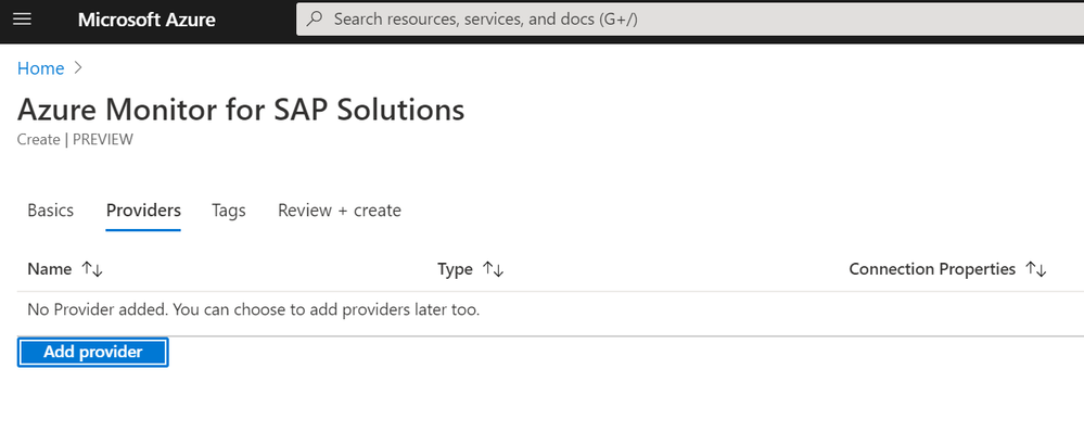
• When finished, select Add provider

As an example, here is a subscription with three clusters – one for NFS, one for SAP HANA, and one for SAP central services. The provider view looks like this:

Overview of the new views

Continuing with the example of the resource group with three clusters, here is the overall HA cluster status:

Here, you can tell that there are three clusters, but only one of them (the NFS cluster) is in a healthy state. The H10 cluster is in maintenance mode, which means the cluster is not managing cluster resources. The s40 cluster has had errors in the resource state.

Cli location constraints

When you select one of the cluster hexagons, you will see more information on that specific cluster. First, there is information on cli-ban or cli-prefer location constraints in the cluster configuration. These constraints are created by commands such as crm resource move or crm resource migrate. This is what you will see in the HA workbook if there are no such constraints:

If there are any of these constraints, you will see the constraint names:

You should remove these constraints after the resource movement has been completed using the “crm configure delete <constraint name>” command. If you do not, they will impact the expected operation of the cluster.

Node status over time

In the cluster view, you will see the current node status for each node in the cluster, and you will now also see the historical status of a particular node at the bottom:

The Time range and node are selectable in this view. This is useful to see when a particular node went offline from the standpoint of the cluster. It will also indicate which of the nodes is the clusters “designated coordinator”.

Resource status over time

The cluster view will show the current resource status for the cluster managed resources, and there is now a historical view of the failure counts for a selected resource:

Again, the time range and resource are selectable in this view. It shows the failure count and failure threshold for the selected resource – If the failure count reaches the threshold, the resource will be moved to another node. Any errors should be investigated and resolved if possible.

Resources

Here are some additional resource links for learning about Azure Monitor for SAP Solutions and providers for other monitoring information:

• Latest updates on AMS


• AMS announcement


• AMS Official documentation


• AMS quick start video


• SAP NetWeaver podcast


• AMS Azure Friday video


• AMS podcast


• AMS integration with Azure Lighthouse for telemetry across tenants


• AMS & SUSE collaboration on AMS

Feedback form:

• AMS asks & feedback form

Summary

We hope you will find the new visualizations helpful, and please let us know if you have ideas for any new features for Azure Monitor for SAP solutions.

Six reasons to join us at RedisConf 2021

by Contributed | Apr 14, 2021 | Technology

This article is contributed. See the original author and article here.

Spring has arrived, which means that RedisConf—the annual celebration of all things Redis—is almost here! Attending RedisConf is one of the best ways to sharpen your Redis skills by exploring best practices, learning about new features, and hearing from industry experts. You’ll also be able to virtually hang out with and learn from thousands of other developers passionate about Redis.

We love Redis here at Microsoft, so we’re excited to be showing up at RedisConf in a big way this year. We’ll not only be talking more about our new Azure Cache for Redis Enterprise offering, but we’ll also be hosting sessions and panels that dive deeper into the best ways to use Redis on Azure. Want to learn more? Here are seven reasons to attend RedisConf 2021:

1. Explore live and on-demand training on how to use Redis with popular frameworks like Spring and .NET Core.


2. Hear Microsoft CVP Julia Liuson present a keynote status update about the ongoing collaboration between Microsoft and Redis Labs, including the Enterprise tiers of Azure Cache for Redis.


3. Listen to customers like Genesys, Adobe, and SitePro who are using Redis Enterprise on Azure for use-cases as diverse as IoT data ingestion and mobile push notification deduplication.


4. Tune in for a roundtable discussion between the Microsoft and Redis Labs teams that touches on what the collaboration between the companies looks like and the benefits it brings to customers.


5. Learn how to harness the power of Redis and Apache Kafka to crunch high-velocity time series data through the power of RedisTimeSeries.


6. Hear from experts from our product team on the best way to run Redis on Azure, including tips-and-tricks for maximizing performance, ensuring network security, limiting costs, and building enterprise-scale deployments.

RedisConf kicks off on April 20^th, and registration is free!  Sign-up now to attend. We’ll see you there.

Making MsQuic Blazing Fast

by Contributed | Apr 14, 2021 | Technology

This article is contributed. See the original author and article here.

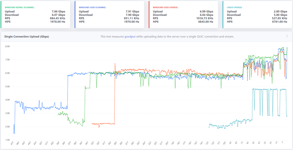
It’s been a year since we open sourced MsQuic and a lot has happened since then, both in the industry (QUIC v1 in the final stages) and in MsQuic. As far as MsQuic goes, we’ve been hard at work adding new features, improving stability and more; but improving performance has been one of our primary ongoing efforts. MsQuic recently passed the 1000^th commit mark, with nearly 200 of those for PRs related to performance work. We’ve improved single connection upload speeds from 1.67 Gbps in July 2020 to as high as 7.99 Gbps with the latest builds*.

* Windows Preview OS builds; User-mode using Schannel; and server-class hardware with USO.
** x-axis above reflects the number of Git commits back from HEAD.

Defining Performance

“Performance” means a lot of different things to different people. When we talk with Windows file sharing (SMB), it’s always about single connection, bulk throughput. How many gigabits per second can you upload or download? With HTTP, more often it’s about the maximum number of requests per second (RPS) a server can handle, or the per-request latency values. How many microseconds of latency do you add to a request? For a general purpose QUIC solution, all of these are important to us. But even these different scenarios can have ambiguity in their definition. That’s why we’re working to standardize the process by which we measure the various performance scenarios. Not only does this provide a very clear message of what exactly is being measured and how, but it has also allowed for us to do cross-implementation performance testing. Four other implementations (that we know of) have implemented the “perf” protocol we’ve defined.

Performance-First Design

As already mentioned above, performance has been a primary focus of our efforts. Since the very start of our work on QUIC, we’ve had both HTTP and SMB scenarios driving pretty much every design decision we’ve made. It comes down to the following: The design must be both performant for a single operation and highly parallelizable for many. For SMB, a few connections must be able to achieve extremely high throughput. On the other hand, HTTP needs to support tens of thousands of parallel connections/requests with very low latency.

This design initially led to significant improvements at the UDP layer. We added support for UDP send segmentation and receive coalescing. Together, these interfaces allow a user mode app to batch UDP payloads into large contiguous buffers that only need to traverse the networking stack once per batch, opposed to once per datagram. This greatly increased bulk throughput of UDP datagrams for user mode.

These design requirements have led to some significant complexity internal to MsQuic as well. The QUIC protocol and the UDP (and below) work are separated onto their own threads. In scenarios with a small number of connections, these threads generally spread to separate processors, allowing for higher throughput. In scenarios with a large number of connections, effectively saturating all the processors with work, we do additional work improves parallelization.

Those are just a few of the (bigger) impacts our performance-driven design has had on MsQuic architecture. This design process has affected every part of MsQuic from the API down to the platform abstraction layer.

Making Performance Testing Integral to CI

Claiming a performant design means nothing without data to back it up. Additionally, we found that occasional, mostly manual, performance testing led to even more issues. First off, to be able to make reasonable comparisons of performance results, we needed to reduce the number of factors that might affect the results. We found that having a manual process added a lot of variability to the results because of the significant setup and tool complexity. Removing the “middleman” was super important, but frequent testing has been even more important. If we only tested once a month, it was next to impossible to identify the cause of any regressions found in the latest results; let alone prevent them from happening in the first place. That inevitably led to a significant amount of wasted time trying to track down the problem. All the while, we had regressed performance for anyone using the code in the meantime.

For these reasons, we’ve invested significant resources into making performance testing a first-class citizen in our CI automation. We run the full performance suite of tests for every single PR, every commit to main, and for every release branch. If a pull request affects performance, we know before it’s even merged into main. If it regresses performance, it’s not merged. With this system in place, we have pretty much guaranteed performance in main will only go up. This has also allowed us to confidently take external contributions to the code without fear of any regressions.

Another significant part of this automation is generating our Performance Dashboard. Every run of our CI pipeline for commits to main generates a new data point and automatically updates the data on the dashboard. The main page is designed to give a quick look at the current state of the system and any recent changes. There are various other pages that can be used to drill down into the data.

Progress So Far

As indicated in the chart at the beginning, we’ve had lots of improvements in performance over the last year. One nice feature of the dashboard is the ability to click on a data point and get linked directly to the relevant Git commit used. This allows us to easily find what code change caused the impacted performance. Below is a list of just a few of the recent commits that had the biggest impact on single connection upload performance.

• d985d44 – Improves the flow control tuning logic


• 1f4bfd7 – Refactors the perf tool


• ec6a3c0 – Fix a kernel issue related to starving NIC packet buffers


• be57c4a – Refactors how we use RSS processor to schedule work


• 084d034 – Refactors OpenSSL crypto abstraction layer


• 9f10e02 – Switches to OpenSSL 1.1.1 branch instead of 3.0


• ee9fc96 – Adds GSO support to Linux data path abstraction


• a5e67c3 – Refactors UDP send logic to run on data path thread

Most of these changes came about from this simple process:

1. Collect performance traces.


2. Analyze traces for bottlenecks.


3. Improve biggest bottleneck.


4. Test for regressions.


5. Repeat.

This is a constantly ongoing process to always improve performance. We’ve done considerable work to make parts of this process easier. For instance, we’ve created our own WPA plugin for analyzing MsQuic performance traces. We also continue to spend time stabilizing our existing performance so that we can better catch possible regressions going forward.

Future Work

We’ve done a lot of work so far and come a long way, but the push for improved performance is never ending. There’s always another bottleneck to improve/eliminate. There’s always a little better/faster way of doing things. There’s always more tooling that can be created to improve the overall process. We will continue to put effort into all these.

Going forward, we want to investigate additional hardware offloads and software optimization techniques. We want to build upon the work going on in the ecosystem and help to standardize these optimizations and integrate it them into the OS platform and then into MsQuic. Our hope is that we will make MsQuic the first choice for customer workloads by bringing the network performance benefits QUIC promises without having to make a trade-off with computational efficiency.

As always, for more info on MsQuic continue reading on GitHub.

Royal Bank of Canada using Always Encrypted with secure enclaves

by Contributed | Apr 14, 2021 | Technology

This article is contributed. See the original author and article here.

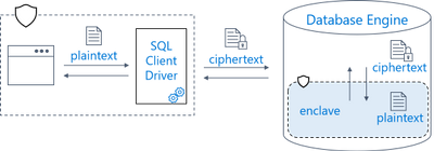
Earlier this year, we announced the preview of Always Encrypted with secure enclaves in Azure SQL Database – the feature designed to safeguard sensitive data from malware and unauthorized users by enabling rich confidential queries.

Royal Bank of Canada (RBC) is one of the customers who are already using Always Encrypted with secure enclaves. For details, see Microsoft Customer Story – RBC creates relevant personalized offers while protecting data privacy with Azure confidential computing.

For more information about Always Encrypted with secure enclaves in Azure SQL Database, see:

• Inside Azure Datacenter Architecture with Mark Russinovich (the segment on Always Encrypted)


• A webinar including a deep dive on Always Encrypted with secure enclaves


• Tutorial: Getting started with Always Encrypted with secure enclaves in Azure SQL Database


• Always Encrypted with secure enclaves – documentation