March ahead with Azure Purview: Setting up scans

by Contributed | Mar 16, 2021 | Technology

This article is contributed. See the original author and article here.

Welcome to the “March Ahead with Azure Purview” blog series that helps you to maximize your Azure Purview trial/pilot/PoC with best practices, tips and tricks from product experts. In the previous blog post, we covered setting up the appropriate control plane and data plane roles to manage Azure Purview. In this post, we’ll roll up the sleeves and walk through the process of scanning data. Let’s get started!

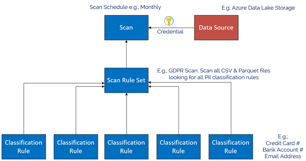
The Azure Purview Data Map enables you to create a holistic knowledge graph of your data residing in on-premises, multicloud and SaaS data stores via automated scanning and classification. The anatomy of an Azure Purview scan involves a number of key components illustrated in this diagram;

Starting at the bottom, we have Classification rules. Out of the box, Purview provides rules for common Personally Identifiable Information (PII) data such as Name, Email Address, Social Security Number and a heap of others. These are known as “System Rules”. We can access the System Rules by clicking Classification Rules in the Management Centre of Purview Studio.

Beyond these, you can create your own custom classification rules using Regular Expressions and Dictionary Lists. Click on the Custom tab and then click + New to add a new Custom Rule. An example below is for Australian Phone Numbers.

Once we have our Classification Rules, we group them together into Scan rule sets, used by a scan to look for certain data points. Out of the box, Purview has default Scan Rule Sets for each Source Type. For example, the default Scan Rule Set for Azure Data Lake Storage Gen 2 will scan all common file types (csv, json, parquet etc) looking for all out of the box System Rules.

You can create your own Scan Rule Sets should you wish to customize how scans are performed. For example, you may only wish to scan certain file types, and include custom classification rules and/or ignore some System rules. This allows you to fine tune the time scans take, and therefore control the cost of Purview. Like Classification Rules, to create a custom Scan Rule Set, click on the Custom tab and then + New.

In the example below, we limit the file types for our custom Scan Rule Set to Parquet and CSV and choose specific classification rules to include in the scan.

Now we have our Classification Rules and Scan Rule Sets, let’s create a data source to scan! On the Sources tab, we click Register, and choose a data source type. Today we natively support a range of Azure data sources such as Azure SQL Database, Power B I and Data Lake Storage, along with preview support for Oracle, SAP and Teradata . This list will expand as we move towards General Availability. Note that for Power BI and 3rd Party data sources such as Oracle, it’s a meta-data only scan. For these sources, we don’t use the classification rules during scanning to detect data such as email addresses.

In my case, I chose Azure Data Lake Storage Gen2, so I’m asked for the account details, such as Subscription, Storage Account Name and what collection on the Data Map I want to register this source into, for example, EnterpriseDataLake.

Once registered, I can now perform a scan of the source by clicking the scan icon.

The first thing I need to do is choose what credentials Purview will use to scan the source. In the example above, I’m using the Purview Managed Service Identity (MSI), so I would need to grant the MSI permissions to read the storage account.

Let’s say my data source was Azure SQL Database, and I wanted to use a username and password, instead of the Purview MSI. In this case, I can choose to create a new credential and use Purview’s integration with Azure Key Vault to securely reference credentials from there.

Depending on the Data Source, the next step asks for the scan scope. In the case of a Data Lake storage account, it might be to select which folders to scan or for a SQL Database, which tables to scan. After this, you choose the Scan Rule Set, as we covered above. In this example I’m choosing my Custom Scan Rule set.

The final step is to choose the scan schedule, which can be either recurring, or a Once-off scan.

And that’s it! The scan is now scheduled to execute per your instructions. You can view the scan status by clicking View details button in the Data Map.

The Details screen shows the scan history and the number of assets scanned and classified.

Once your scan completes, you can browse the assets from the home page, using either the Search bar, or the Browse Assets button.

Depending on the source, the scan setup process varies, for example, On-Premises SQL Server, AWS S3, Teradata, Oracle, SAP S/4HANA and SAP ECC. And be sure to checkout this blog post, which covers additional information on scanning, including Resource sets and scanning scale.

Finally, we’ve encapsulated some important Purview best practices here covering stakeholder management, deployment models and platform hardening.

Happy scanning!

Managed and External table on Serverless

by Contributed | Mar 16, 2021 | Technology

This article is contributed. See the original author and article here.

The purpose of this about is to discuss Managed and External tables while querying from SQL On-demand or Serverless.

Thanks to my colleague Dibakar Dharchoudhury for the really nice discussion related to this subject.

By the docs: Shared metadata tables – Azure Synapse Analytics | Microsoft Docs

• Managed tables

Spark provides many options for how to store data in managed tables, such as TEXT, CSV, JSON, JDBC, PARQUET, ORC, HIVE, DELTA, and LIBSVM. These files are normally stored in the warehouse directory where managed table data is stored.

• External tables

Spark also provides ways to create external tables over existing data, either by providing the LOCATION option or using the Hive format. Such external tables can be over a variety of data formats, including Parquet.

Azure Synapse currently only shares managed and external Spark tables that store their data in Parquet format with the SQL engines

Note “The Spark created, managed, and external tables are also made available as external tables with the same name in the corresponding synchronized database in serverless SQL pool.”

Following an example of an External Table created on Spark-based in a parquet file:

1) Authentication:

blob_account_name = "StorageAccount"
blob_container_name = "ContainerName"
from pyspark.sql import SparkSession

sc = SparkSession.builder.getOrCreate()
token_library = sc._jvm.com.microsoft.azure.synapse.tokenlibrary.TokenLibrary
blob_sas_token = token_library.getConnectionString("LInkedServerName")

spark.conf.set(
    'fs.azure.sas.%s.%s.blob.core.windows.net' % (blob_container_name, blob_account_name),
    blob_sas_token)

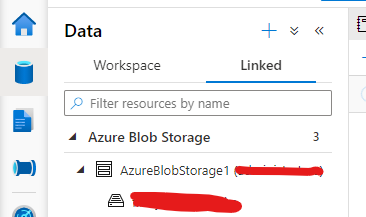
Note my linked Server Configuration:

2) External table:

Spark.sql('CREATE DATABASE IF NOT EXISTS SeverlessDB')

#THE BELOW EXTERNAL SPARK TABLE 
filepath ='wasbs://Container@StorageAccount.blob.core.windows.net/parquets/file.snappy.parquet'
df = spark.read.load(filepath, format='parquet')
df.write.mode('overwrite').saveAsTable('SeverlessDB.Externaltable')

 Here you can query from SQL Serverless

If you check the path where your external table was created you will be able to see under the Data lake as follows.  For example, my workspace name is synapseworkspace12:

3) I can also create a managed table as parquet using the same dataset that I used for the external one as follows:

#Managed - table
df.write.format("Parquet").saveAsTable("SeverlessDB.ManagedTable")

CREATE TABLE SeverlessDB.myparquettable(id int, name string, birthdate date) USING Parquet

-- Drop the database and it's tables
DROP DATABASE SeverlessDB CASCADE

Team21 – A hackathon story AI Hack 2021 Kaiko Cryptocurrency Challenge Winners

by Contributed | Mar 16, 2021 | Technology

This article is contributed. See the original author and article here.

Introduction & Profiles

Hi there everyone! We are Team 21, first place prize winners of the Imperial College London Data Science Society’s (ICDSS) 2021 AI Hackathon for the ‘Kaiko Cryptocurrency Challenge’. We are Howard, a penultimate Mechanical Engineering student and Stephanie, a penultimate Molecular Bioengineering student from Imperial College London.

Check out the full report and code in this repo: https://github.com/howardwong97/AI-Hack-2021-Team-21-Submission .

Feel free to contact us if you have any questions!

	Linkedin: https://www.linkedin.com/in/howardwongjy/ GitHub: https://github.com/howardwong97
	Linkedin: https://www.linkedin.com/in/stephaniesze/ GitHub: https://github.com/steph128

Kaiko Cryptocurrency Challenge and Our Motivation

The Kaiko Cryptocurrency Challenge provided cryptocurrency market data to create a predictive model. We tackled this challenge by investigating the effectiveness of traditional time series models in predicting volatility in the cryptocurrency market and the effect of introducing social media sentiment.  

If we look at the Bitcoin volatility index, the latest 30-day estimate for the BTC/USD pair is 4.30%. There are several factors contributing to the high volatility in cryptocurrency prices: low liquidity, minimal regulation, and the fact that it’s a very young market. It is incredibly difficult to apply fundamental analysis and so the values of cryptocurrencies are mostly driven by speculation. Social media, therefore, makes a huge impact. Take the tweet from Elon Musk about Dogecoin, for example, we observed a dramatic price drop and increased volatility. Although we can’t say with certainty that what happened was a direct result of the tweet, we cannot underestimate the effect of social media on the cryptocurrency market.

Exploratory Data Analysis

Instead of working directly with prices, we compute the returns, which normalizes the data to provide a comparable metric. Furthermore, we take the log of the returns, which has the desirable property of additivity. Denoted by , the log returns can be written as

The histogram of log returns is plotted below. It is often assumed that log returns, especially in the equities market, are normally distributed. The unimodal distribution seems to agree with this assumption. However, the negative skew and excess kurtosis suggests that this is not the case!

We are interested in modelling the serial correlation observed in the log returns. The autocorrelation function (ACF) plot suggests that there is significant serial correlation. In addition, plotting the partial autocorrelation function (PACF) of the squared log returns allows shows autoregressive conditional heteroskedastic effects (more on this later). In other words, the volatility is not serially independent.

Lastly, we talk about the concept of stationarity. Roughly speaking, a time series is said to be weakly stationary if both the mean of   and the covariance of  and   are time invariant. This is the foundation of time series analysis; the mean is only informative if the expected value remains constant across time periods. Therefore, we performed the Augmented Dickey-Fuller unit-root test and confirmed that the log returns is indeed stationary.

Time Series Analysis

A mixed autoregressive moving average process, or ARMA, is written as

One of the assumptions of ARMA is that the error process, , is homoscedastic or constant over time. However, we have seen from the PACF plot of the squared log returns that this might not be the case. Volatility has some interesting characteristics. Firstly, asset returns tend to exhibit volatility clustering; volatility tends to remain high (or low) over long periods. Secondly, volatility evolves in a continuous manner; large jumps in volatility are rare. This is where volatility models come in. The idea of autoregressive conditional heteroscedasticity (ARCH) is that the variance of the current error term  is dependent on previous shocks. An ARCH model assumes.

Generalised ARCH (GARCH) builds upon ARCH by allowing lagged conditional variances to enter the model as well:

The constants ,   and  are parameters to be estimated.  can be interpreted as a measure of the reaction of the volatility to market shocks, while  measures its persistence. Therefore, ARMA specifies the structure of the conditional mean of log returns, while GARCH specifies the structure of the conditional variance. Put together, an ARMA-GARCH can be summarised as

Forecasting Volatility

Another interesting property of volatility is that it is not directly observable. For example, if we had daily log returns data for BTC, we cannot establish the daily volatility. However, data with finer granularity (e.g., one-minute data) is available, one can estimate this by taking the sample standard deviation over a single trading day. Therefore, we used the following forecasting scheme:

1. Reduce the resolution of the log returns to five-minute intervals. Since log returns are additive, we can simply sum the log returns   to  .


2. Compute the realized volatility for each five-minute period.


3. Use a rolling window of 120 samples to fit ARMA-GARCH using maximum likelihood.


4. Use fitted parameter estimates to compute the forecasted volatility for the next five-minute interval.

Fitting the model on a rolling window and then forecasting the following period’s five-minute volatility ensure that we avoid look-ahead bias.

The results are plotted above. Clearly, the ARMA GARCH model did not perform very well! Indeed, we have fitted ARMA(1,1) and GARCH(1,1) for simplicity; other lag orders could be necessary. One could also argue that the models were also over a relatively short timeframe.

Sentiment Analysis

There are many flavours of GARCH (e.g. I-GARCH, E-GARCH). However, we are interested in exploring the possibility of introducing sentiment regressors to the GARCH model specification. It is straightforward to introduce additional terms, i.e.

where   is an additional explanatory variable, and  is a new parameter to be estimated.

So how do we measure sentiment? For this, we turn to Reddit, which provides an API for searching for posts and comments. We performed a search for “Bitcoin” and “BTC” across several subreddits (yes, including WallStreetBets).

What remains is to engineer features for our model. There are two key features that we saw to be the most informative:

• Frequency – how many times Bitcoin has been mentioned on Reddit within a timeframe?


• Sentiment – what is the overall sentiment (positive or negative)?

Indeed, upvotes would have been a good feature to include too, as it is an indication of the reach of the post or comment. However, we did not include this in this project.

Natural Language Processing (NLP) techniques have been utilised in the past to detect sentiment as positive or negative. However, comments about the financial markets are unique in terms of terminology. Therefore, a domain-specific corpus must be built to train a sentiment model. Conveniently, Stocktwits is a site where users can label their own comments as either “bullish” or “bearish”, so this would be the perfect source for training data. In our past work, we scraped thousands of posts and trained a RoBERTa model.

What is RoBERTa? Many are familiar with BERT, the self-supervised method released by Google in 2018. Researchers at the University of Washington built upon this by removing BERT’s next-sentence pretraining objective, and training with much larger mini-batches and learning rates. We chose this due to its promise of better downstream task performance – this is especially important in a 24-hour Hackathon!

Feature Engineering

Having scraped all mentions of Bitcoin on Reddit over the period, we made sentiment predictions using our financial RoBERTa model, which labels each comment as “Bullish” (positive) or “Bearish” (negative). We created the following features:

• N, the number of comments made about BTC in the past hour.


• S, computed by defining  and  and summing these for each comment in the past hour.

The new GARCH specification is now

It is important to ensure that N and S are synchronous with the log returns (i.e. the post or comment was published at or before the time period of interest).

 Results

So, how did our new sentiment-based model perform? Terribly! In fact, the mean square error (MSE) of this new model was about ten times worse than the original model. There are clearly many pitfalls in the work that we have presented here. Our sentiment model was clearly very simplistic as it only provided a ‘bullish’ or ‘bearish’ signal. The Reddit dataset that we created was also relatively small – there are other sources of news that we could have used. One could also argue that our sentiment model was incapable of identifying bots deployed to manipulate sentiment models such as this one.

Something also must be said about the efficacy of traditional time series models. GARCH models have historically been rather effective in forecasting daily volatility. However, our intuition tells us that social media sentiment clearly plays a big factor. Our future work will be focused on thinking of more appropriate ways of integrating this into our model.

Resources 
Microsoft Learn BlockChain 
Beginners Guide to BlockChain on Azure

Microsoft 365 PnP Weekly – Episode 118

by Contributed | Mar 16, 2021 | Technology

This article is contributed. See the original author and article here.

In this installment of the weekly discussion revolving around the latest news and topics on Microsoft 365, hosts – Vesa Juvonen (Microsoft) | @vesajuvonen, Waldek Mastykarz (Microsoft) | @waldekm are joined by are joined by Scotland-based Solution Architect, dual MVP Veronique Lengelle (CPS) | @veronicageek.  

The discussion included insights to the role of technical architect for Microsoft 365 platform – both about designing solutions that solve customer problems and as important – educating customers on the value of the integrated platform.  Microsoft Teams vs SharePoint – meet the customer where they are at and coach from there.  “Don’t neglect to deliver SharePoint training and don’t focus solely on Microsoft Teams.”  And finally, the growth in partner opportunities as many customers who quickly moved to M365 and the cloud in the last year are now looking for guidance on how to leverage many more of the platform’s capabilities that they own.   Veronique is an active contributor to PnP PowerShell project, as a champion for Sys Admin users.   

As with the previous week, Microsoft and the Community delivered 23 articles and videos this last week.  Brilliant!  This session was recorded on Monday, March 15, 2021.  

This episode was recorded on Monday, March 15, 2021.

• Video at Microsoft 365 Community YouTube channel.


• Podcast format at https://pnpweekly.podbean.com.

These videos and podcasts are published each week and are intended to be roughly 45 – 60 minutes in length.  Please do give us feedback on this video and podcast series and also do let us know if you have done something cool/useful so that we can cover that in the next weekly summary! The easiest way to let us know is to share your work on Twitter and add the hashtag #PnPWeekly. We are always on the lookout for refreshingly new content. “Sharing is caring!”

Here are all the links and people mentioned in this recording. Thanks, everyone for your contributions to the community!

Microsoft articles:

• Four device capabilities developers can utilize for Microsoft Teams mobile apps – Microsoft


• Microsoft Graph Mailbag – Microsoft Graph in Electron applications using Microsoft Graph Toolkit – Microsoft


• Microsoft Graph Toolkit adds a new Electron Provider plus enhanced capabilities – Microsoft


• GlobalCon5 – three days of sessions and workshops – Mark Kashman (Microsoft) | @mkashman


• 11 New Connectors Released in February 2021! – Doug Elliott (Microsoft) 


• How to implement document automation in your business with Microsoft Power Platform – Cedrick Bellarosa (Microsoft)


• Microsoft 365 Extensibility look book gallery – Microsoft 

Community articles:

• Microsoft 365 Community (PnP) – March 2021 update – Vesa Juvonen (Microsoft) | @vesajuvonen


• Getting started with PnP Core SDK – Paul Bullock (CaPa Creative) | @pkbullock


• Getting started with SharePoint’s custom column formatting – Will Holland (ThreeWill) | @_wcholland


• Run CLI for Microsoft 365 in Docker – Garry Trinder (CPS) | @garrytrinder


• 10 things we should think about before we build an app – Luise Freese | @LuiseFreese


• 5 commands to try in CLI for Microsoft 365 to fall in love with it – Luise Freese | @LuiseFreese


• Doctor – Maintain your documentation on SharePoint without pain – Elio Struyf (Struyf Consulting) | @eliostruyf


• Init API permissions for your SPFx projects without deploying them – Michaël Maillot (onepoint) | @michael_maillot


• Getting started with SharePoint Framework – Waldek Mastykarz (Microsoft) | @waldekm


• Episode #145​ – Welcome PnP Core SDK! – Paolo Pialorsi (PiaSys) | @PaoloPia


• SharePoint Framework for beginners (SPFx) 2021 | Episode 02 – Development Environment – Rob Pearmain (yorcloud) | @robertpearmain


• Migration report with CLI for Microsoft 365 – Albert-Jan Schot (Portiva) | @appieschot


• Building Outlook addin with SPFx – save mail to OneDrive with Azure Function, MSAL.NET and MS Graph .NET – Sergei Sergeev (Mastaq) | @sergeev_srg


• Export external users with CLI for Microsoft 365 – Albert-Jan Schot (Portiva) | @appieschot


• Should you use a default label with Microsoft Information Protection (MIP)? – Sarah Haase | @sarahhaase, Antonio Maio | @AntonioMaio2 and Mike Maadarani | @mikemaadarani


• SharePoint Form Conditional Formulas – Laura Rogers (IW Mentor) | @WonderLaura

Additional resources:

• PnP Sharing is Caring initiative – Getting started guidance and training for using GitHub and contributing to the community


• Want to ask a question or in general engage with the community – Add a note in the Microsoft 365 PnP Community hub at https://aka.ms/m365pnp/community


• Check out all the great community calls, SDKs, and tooling for Microsoft 365 from https://aka.ms/m365pnp

If you’d like to hear from a specific community member in an upcoming recording and/or have specific questions for Microsoft 365 engineering or visitors – please let us know. We will do our best to address your requests or questions.

“Sharing is caring!”