Power BI Reports for Azure Lab Services – Part 1: Visualizing Cost Management Data

by Contributed | Aug 18, 2021 | Technology

This article is contributed. See the original author and article here.

Azure Lab Services costs are integrated with Cost Management on the lab account level.  However, sometimes it’s useful to create a custom report for your team.  We can do this using the line item data from Cost Management.  In this blog post we will use Power BI desktop to create a basic report that shows total cost, total number of virtual machines and total number of labs.  The report will also include a table that shows cost per lab and cost per virtual machine.

To create this report, we need to complete four major tasks.

1. Get the data. We need to import data into PowerBI.


2. Transform the data.   Each cost line item has all the information we need, but it will need to be separated, so we can work with lab and lab virtual machine information individually.


3. Create the data visualization.


4. Publish the report for others to see.

Get the data

There are couple options to import the Cost Management data into PowerBI.  Which one to use will depend on your type of Azure agreement and your permission level.

Azure Cost Management connector

The first option is the Azure Cost Management connector. Follow the instructions at Create visuals and reports with the Azure Cost Management connector in Power BI Desktop.  You will need to provide a billing scope which could cover from a billing agreement to a specific resource group.  See understand and work with Azure Cost Management scopes for more information about scopes.  See identify resource id for a scope for instructions to get billing scope based on the type of scope you are using.

The Azure Cost Management connector currently supports customers with a Microsoft Customer Agreement or an Enterprise Agreement (EA).  There are also some unsupported subscription types.  To successfully use the connector, you must have correct permissions and the ability for users to read cost management data must be enabled by the tenant administrator.  You can check your access by calling the cost management usage detail api directly.

Azure Cost Management exports

The second option is to export costs to a storage account fromAzure Cost Management.  Follow instructions at Tutorial – Create and manage exported data from Azure Cost Management | Microsoft Docs to create the recurring export.  You can choose to have data exported daily, weekly or monthly.  Each export will be a CSV file saved in blob storage.

In PowerBI Desktop, we will use the Azure Blob Storage connector to import this data.  Select the usage detail data from the storage account container you used when scheduling the cost management data exports.  Choose to combine the files when importing the CSV file data.

Transform the data

Each usage detail line item has the information for the full resource id of the virtual machine (either template or student) associated with the cost.  As explained in cost management guide for Azure Lab Services, these resources will follow one of two patterns. 

For templates virtual machines:

/subscriptions/{subscription-id}/resourceGroups/{resource-group}/providers/Microsoft.LabServices/labaccounts/{lab-account-name}/environmentsettings/default

For student virtual machines:

/subscriptions/{subscription-id}/resourceGroups/{resource-group}/providers/Microsoft.LabServices/labaccounts/{lab-account-name}/environmentsettings/default/environments/{vm-name}

For our report, we will need to extract the required data the from the InstanceId property of the Cost Management usage details.  Complete the following steps in Power Query.

1. Filter on ConsumedService equal to microsoft.labservices. 


2. Remove duplicate rows.  We do this to avoid any issues if using Cost Management exports and data is accidentally exported multiple times.  Select all columns except the Source.Name.


3. Duplicate InstanceId column and rename it ResourceId.


4. Split the InstanceId column on the ‘/’ character.


5. Clean up split columns.
   
   
   
   8. Delete InstanceId.1 to InstanceId.8.  We already have the SubscriptionGuid and ResourceGroup columns, so the InstanceId.3 and InstanceId.5 columns aren’t needed. 
   
   
   9. Rename InstanceId.9 to LabAccount.
   
   
   10. Delete InstanceId.10.
   
   
   11. Rename InstanceId.11 to Lab.
   
   
   12. Delete InstanceId.12 to InstanceId.14.
   
   
   13. Rename InstanceId.15 to VirtualMachine.
   
   
   14. Replace ‘null’ values with ‘template’.  Any rows that don’t have a value for VirtualMachine are costs associated with running the template virtual machine for the lab.
   
   
   
   


6. Save transformations.

Schema for the table should look something like the picture below.  Depending on your Azure subscription type, there may be more columns not seen in this example.

Visualize the data

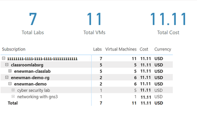
First, let’s create some cards for high-level information.  Our cards will show the total cost, number of labs and number of virtual machines used. 

Total Cost

The total cost is held in the PreTaxCost column.  PowerBI already recognizes that PreTaxCost is number and will automatically add all the column values to create a sum.  Add a card to the visual and add PreTaxCost to the Field property of the card visualization.  Optionally change the name for the visualization from PreTaxCost to Total Cost.  

Number of Labs

Next, let’s display the number labs.  We’ll need to create a new measure for this.  For instructions explaining how to create a new measure, see create your own measures in Power BI Desktop tutorial. 

For the most accurate reporting, we can’t just create a measure that counts all the distinct values in the Lab column because it is possible to have two labs with the same name in different lab accounts.  So, for our measure named NumberOfLabs we will count the number of rows when grouped by all the identifying columns for a lab, which are subscription, resource group, lab account and lab name.  Note, in this example the table name is dailyexports.

NumberOfLabs = COUNTROWS(GROUPBY(dailyexports, dailyexports[SubscriptionGuid], dailyexports[ResourceGroup], dailyexports[LabAccount], dailyexports[Lab]))

Now we can create a card for the NumberOfLabs measure by following instructions at create card visualizations (big number tiles).

Total Number of Virtual Machines

Creating a card for the total number of virtual machines used will be similar to creating a card for total number of labs.  We need to create a measure that counts the unique combination of subscription, resource group, lab account, lab and virtual machine name.  Our new measure is

NumberOfVMs = COUNTROWS(GROUPBY(dailyexports, dailyexports[SubscriptionGuid], dailyexports[ResourceGroup], dailyexports[LabAccount], dailyexports[Lab], dailyexports[VirtualMachine]))

Now we can create a card for NumberOfVMs measure by following instructions at create card visualizations (big number tiles) .

Matrix

Now let’s create a matrix visual to allow us to drill down into our data. For instructions how to create a matrix visualization, see create a matrix visual in Power BI.  For our matrix visualization, we’ll add the Subscription, ResourceGroup, Lab Account, Lab, VirtualMachine for the rows.  NumberOfLabs, NumberOfVMs, PreTaxCost and Currency will be our values.  Note, for the currency column, the first value for currency will be shown with the matrix is collapsed.

After of renaming the columns for the visuals and applying some theming, our report now looks like the following picture.  I’ve expanded the subscription, resource groups and the ‘enewman-demo’ lab account.  Under the lab account you can see the two labs and total cost for each lab.  As you can see by the plus sign next to the lab’s names, each lab could be expanded to list the virtual machines for the lab as well as the cost for each virtual machine.

Publish the data

Last step is to publish the report!  See publish datasets and reports from Power BI Desktop for further instructions.

Happing Reporting!

The Lab Services Team

Azure VMware Solution Releases Placement Polices in Public Preview

by Contributed | Aug 16, 2021 | Technology

This article is contributed. See the original author and article here.

Co-Authored: Ashwin Kabadi, Senior Product Manager, Azure VMware Solution, Microsoft

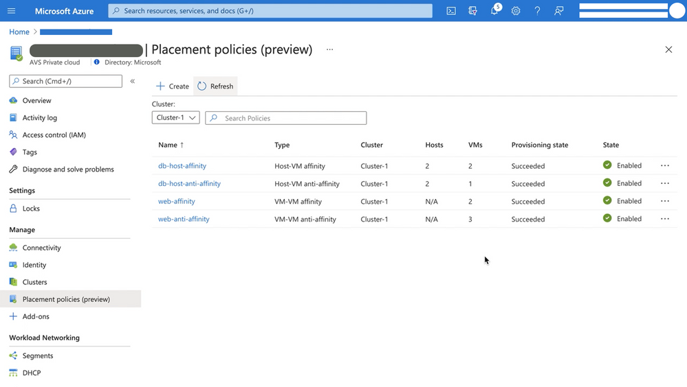
Placement policies enable admins to specify constraints or rules when allocating Virtual Machines within an Azure VMware Solution (AVS) private cloud. With this update the creation and assignment of vSphere Distributed Resource Scheduler (DRS) rules for running Virtual Machines (VMs) in an AVS SDDC has been simplified and is now executable directly from the Azure Portal for cloud admin roles.

Making updates to VM (Virtual Machine) groups and Host groups is a cumbersome operation, especially for hosts in a cloud environment where they can be more frequently cycled. In an on-premises environment, as hosts are replaced in the vSphere inventory, the vSphere admin must modify the host group to ensure that the desired VM-Host placement constraints continue to stay in effect. Placement policies in AVS take care of updating the Host groups when a host is rotated or changed. Similarly, if you scale-in a cluster, the Host Group is also updated automatically, as applicable. This eliminates the overhead of managing the Host Groups.

Placement policies essentially define constraints or rules that allow you to decide where and how the VMs should run within the AVS SDDC clusters. Placement polices are used to support VM performance and availability by grouping multiple VMs that communicate regularly on the same host.  policy and help mitigate the impact of maintenance operations to policies within the SDDC cluster. Placement polices in AVS also reduce the complexity and administrative burden of updating host groups via DRS rules in vSphere during SDDC maintenance operations.

When you create a placement policy, it creates a vSphere Distributed Resource Scheduler (DRS) rule in the specified vSphere cluster. It also includes additional logic for interoperability with Azure VMware Solution operations.

There are two basic placement policy types now supported:

2. Virtual Machine to Virtual Machine: this refers to a policy that is applied to VMs with respect to each other.
   
   
   
   • VM-VM Affinity policies instruct DRS to try keeping the specified VMs together on the same host for performance reasons as an example.
   
   
   • VM-VM Anti-Affinity policies instruct DRS to try keeping the specified VMs apart from each other on separate hosts. It’s useful in scenarios where  you may want to spread your virtual machines across hosts to ensure availability of the applications.
   
   
   
   


3. Virtual Machine to SDDC Host: this refers to a policy applied to selected VMs to either run on, or avoid  selected hosts  .
   
   
   
   • VM-Host Affinity policies instruct DRS to try running the specified VMs on the hosts defined.
   
   
   • VM-Host Anti-Affinity policies instruct DRS to try running the specified VMs on hosts other than those defined.
   
   
   
   

For more information on requirements for placement policies in Azure VMware Solution and how to create and apply them, see Microsoft Docs pages here.

Start using placement polices directly from the Azure Portal  today!

Synapse Data Flows Enables Direct Workspace DB Connector

by Contributed | Aug 14, 2021 | Technology

This article is contributed. See the original author and article here.

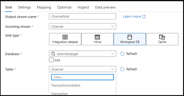
Azure Synapse Analytics Data Flows has enabled Direct Workspace DB Connector as a public preview. This new connector type in data flows enables data engineers to quickly and easily build ETL processes using Spark-based lake databases in Synapse without the need to first create linked services or datasets.

https://docs.microsoft.com/en-us/azure/data-factory/data-flow-source#workspace-db-synapse-workspaces-only

https://docs.microsoft.com/en-us/azure/data-factory/data-flow-sink#workspace-db-synapse-workspaces-only

By using Synapse Analytics for your end-to-end big data analytics projects, you can now define lake database tables using Spark Notebooks, then open the visual data flow designer graph environment and immediately access those tables and data for ETL pipeline building. This new Workspace DB process eliminates the need to create ADF-based linked services and datasets inside of your Synapse workspace studio UI because Synapse is providing the complete integrated experience for data engineers in a single pane of glass.

Microsoft 365 Defender Ninja August 2021 special edition!

by Contributed | Aug 13, 2021 | Technology

This article is contributed. See the original author and article here.

Are you enjoying the summer or winter – wherever you are in the world, and want to keep up to date with the latest and greatest? We can help you cure that need :smiling_face_with_smiling_eyes:

Over the past few months, we have made big product announcements across the Microsoft Defender products and Microsoft Cloud App Security, and of course we want you to stay updated!

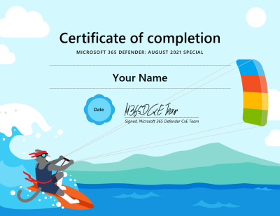
With the following resources you can bring yourself up to speed, and with the knowledge check at the end you can verify your learnings. Plus, you can request either a Ninja summer or winter special edition fun certificate to enrich your Ninja certs collection!

Legend:

Microsoft Defender for Endpoint

Unmanaged devices

•  Unmanaged device protection capabilities


•  Device discovery


•  Endpoint Discovery – Navigating your way through unmanaged devices

Mobile threat defense

•  New capabilities on Android and iOS

Threat and vulnerability management

•  Threat and Vulnerability Management now supports all major platforms


•  Secure configuration assessment for macOS and Linux


•  Vulnerability management for Linux


•  Threat and vulnerability management integrates with ServiceNow VR

Device control

•  Control your USB devices on Mac


•  Device control for MacOS


•  Protect your removable storage and printers

Live response

•  Live response API

Evaluation Lab

•  Renew your lab resources and try new simulations


•  Microsoft Defender for Endpoint evaluation lab

Microsoft 365 Defender:

Threat Analytics

•  Threat analytics


•  Overview of Threat Analytics

Advanced hunting

•  Take action on advanced hunting query results


•  Data tables in the Microsoft 365 Defender advanced hunting schema


•  DeviceFromIP() function in advanced hunting

Integration and APIs

•  Overview of the Streaming API


•  Streaming API Announcement blog


•  Stream Microsoft 365 Defender events


•  Azure Sentinel and Microsoft 365 Defender incident integration


•  Overview Azure Sentinel integration


•  Azure Sentinel integration

 Webinar: Monthly threat insights: New webinar series: Monthly threat insights – Microsoft Tech Community

Defender for Office 365:

Phishing protection

•  Announcing General Availability of Safe Links for Microsoft Teams

Business Email Compromise

•  Business email compromise: How Microsoft is combating this costly threat

Incident investigation

•  Introducing the email entity page


•  Spoof intelligence insight in EOP

Configuration

•  Mastering configuration Part 1


•  Mastering configuration Part 2

 Threat Analytics

•  Threat analytics report tags

Attack Simulation Training

•  Updates to Attack Simulation Training


•  Setting up a New Phish Simulation Program – Part One


•  Setting up a New Phish Simulation Program – Part Two

Defender for Identity:

General:

•  Use Defender for Identity to de-risk your organizations lateral movement paths


•  Make powerful Advanced Hunting queries in Microsoft 365 Defender using Defender for Identity data


•  Deep dive into the latest Defender for Identity detections with the engineering team

Portal Convergence:

•  Portal convergence tracking blog – with the latest updates on what’s happening and when


•  Defender for Identity’s settings and configuration now in Microsoft 365 Defender


•  Microsoft Defender for Identity in Microsoft 365 Defender

Detections

•  Suspected exploitation attempt on Windows Print Spooler service


•  Suspected AS-REP Roasting attack

Identity Security Posture Management assessments

•  Microsoft Defender for Identity legacy protocols identity security posture assessment


•  Microsoft Defender for Identity unconstrained Kerberos identity security posture assessment

Cloud App Security:

3^rd Party Integration

•  How Cloud App Security helps protect your Slack Enterprise


•  How Cloud App Security helps protect your Zendesk


•  How Cloud App Security helps protect your OneLogin

Threat Protection

•  Overview – Advanced hunting


•  The Hunt in a multi-stage incident


•  MCAS: Top 5 Queries You Need to Save


•  Hunting with Microsoft Cloud App Security data

Conditional Access App Control

•  Deploy Cloud App Security Conditional Access App Control for any web app using AD FS


•  Bypass Blocking PDF Previews in OWA

Data Loss Prevention

•  MCAS Data Protection Blog Series: MCAS DLP Walk-Through


•  Integrate Azure Information Protection with Cloud App Security

If you want to verify your learnings, you can participate in this knowledge check.

Once you’ve finished the knowledge check, please click here to request your certificate (you’ll see it in your inbox within a couple of  days.)

Let us know how you like it!

As a reminder, the full Ninja Trainings are here:

Microsoft 365 Defender > http://aka.ms/m365dninja  

Microsoft Defender for Office 365 > https://aka.ms/mdoninja

Microsoft Defender for Endpoint > http://aka.ms/mdeninja

Microsoft Defender for Identity > http://aka.ms/mdininja

Microsoft Cloud App Security > http://aka.ms/mcasninja