
by Contributed | Dec 2, 2021 | Dynamics 365, Microsoft 365, Technology
This article is contributed. See the original author and article here.
You chose Dynamics 365 for your enterprise to improve visibility and to transform your business with insights. Is it a challenge to provide timely insights? Does it take too much effort to build and maintain complex data pipelines?
If your solution includes using a data lake, you can now simplify data pipelines to unlock the insights hidden in that data by connecting your Finance and Operations apps environment with a data lake. With general availability of the Export to Data Lake feature in Finance and Operations apps, data from your Dynamics 365 environment is readily available in Azure Data Lake.
Data lakes are optimized for big data analytics. With a replica of your Dynamics 365 data in the data lake, you can use Microsoft Power BI to create rich operational reports and analytics. Your data engineers can use Spark and other big data technologies to reshape data or to apply machine learning models. Or you can work with a data lake the same way that you work with data in a SQL database. Serverless SQL pool endpoints in Azure Synapse Analytics conveniently lets you query big data in the lake with Transact-SQL (T-SQL).
Why limit yourself to business data? You can ingest legacy data from previous systems as well as data from machines and sensors at a fraction of the cost incurred when storing data in a SQL data warehouse. You can easily mash-up business data with signals from sensors and machines using Azure Synapse Analytics. You can merge signals from the factory floor with production schedules, or you can merge web logs from e-commerce sites with invoices and inventory movement.
Can’t wait to try this feature? Here are the steps you need to follow.
Install the Export to Data Lake feature
The Export to Data Lake feature is an optional add-in included with your subscription to Dynamics 365. This feature is generally available in certain Azure regions: United States, Canada, United Kingdom, Europe, South East Asia, East Asia, Australia, India, and Japan. If your Finance and Operations apps environment is in any of those regions, you can enable this feature in your environment. If your environment isn’t in one of the listed regions, complete the survey and let us know. We will make this feature available in more regions in the future.
To begin to use this feature, your system administrator must first connect your Finance and Operations apps environment with an Azure Data Lake and provide consent to export and use the data.
To install the Export to Data Lake feature, first launch the Microsoft Dynamics Lifecycle Services portal and select the specific environment where you want to enable this feature. When you choose the Export to Data Lake add-in, you also need to provide the location of your data lake. If you have not created a data lake, you can create one in your Azure subscription by following the steps in Install Export to Azure Data Lake add-in.
Choose data to export to a data lake
After the add-in installation is complete, you and your power users can launch the environment for a Finance and Operations app and choose data to be exported to a data lake. You can choose from standard or customized tables and entities. When you choose an entity, the system chooses all the underlying tables that make up the entity, so there is no need to choose tables one by one.
Once you choose data, the system makes an initial copy of the data in the lake. If you chose a large table, the initial copy might take a few minutes. You can see the progress on screen. After the initial full copy is done, the system shows that the table is in a running state. At this point, all the changes occurring in the Finance and Operations apps are updated in the lake.
That’s all there is to it. The system keeps the data fresh, and your users can consume data in the data lake. You can see the status of the exports, including the last refreshed time on the screen.
Work with data in the lake
You’ll find that the data is organized into a rich folder structure within the data lake. Data is sorted by the application area, and then by module. There’s a further breakdown by table type. This rich folder structure makes it easy to organize and secure your data in the lake.
Within each data folder are CSV files that contain the data. The files are updated in place as finance and operations data is modified. In addition, the folders contain metadata that is structured based on the Common Data Model metadata system. This makes it easy for the data to be consumed by Azure Synapse, Power BI, and third-party tools.
If you would like to use T-SQL to work with data in Azure Data Lake, as if you are reading data from a SQL database, you might want to use the CDMUtil tool, available from GitHub. This tool can create an Azure Synapse database. You can query the Synapse database using T-SQL, Spark, or Synapse pipelines as if you are reading from a SQL database.
You can make the data lake into your big data warehouse by bringing data from many different sources. You can use SQL or Spark to combine the data. You can also create pipelines with complex transforms. And then, you can create Power BI reports right within Azure Synapse. Simply choose the database and create a Power BI dataset in one step. Your users can open this dataset in Power BI and create rich reports.
Next steps
Read an Export to Azure Data Lake overview to learn more about the Export to Data Lake feature.
For step-by-step instructions on how to install the Export to Data Lake add-in,see Install Export to Data Lake add-in.
We are excited to release this feature to general availability. You can also join the preview Yammer group to stay in touch with the product team as we continue to improve this feature.
The post Unlock hidden insights in your Finance and Operations data with data lake integration appeared first on Microsoft Dynamics 365 Blog.
Brought to you by Dr. Ware, Microsoft Office 365 Silver Partner, Charleston SC.
by Contributed | Dec 1, 2021 | Technology
This article is contributed. See the original author and article here.
This public preview of Microsoft Azure Active Directory (Azure AD) custom security attributes and user attributes in ABAC (Attribute Based Access Control) conditions builds on the previous public preview of ABAC conditions for Azure Storage. Azure AD custom security attributes (custom attributes, here after) are key-value pairs that can be defined in Azure AD and assigned to Azure AD objects, such as users, service principals (Enterprise Applications) and Azure managed identities. Using custom attributes, you can add business-specific information, such as the user’s cost center or the business unit that owns an enterprise application, and allow specific users to manage those attributes. User attributes can be used in ABAC conditions in Azure Role Assignments to achieve even more fine-grained access control than resource attributes alone. Azure AD custom security attributes require Azure AD Premium licenses.
We created the custom attributes feature based on the feedback we received for managing attributes in Azure AD and ABAC conditions in Azure Role Assignments:
- In some scenarios, you need to store sensitive information about users in Azure AD, and make sure only authorized users can read or manage this information. For example, store each employee’s job level and allow only specific users in human resources to read and manage the attribute.
- You need to categorize and report on enterprise applications with attributes such as the business unit or sensitivity level. For example, track each enterprise application based on the business unit that owns the application.
- You need to improve your security posture by migrating from API access keys and SAS tokens to a centralized and consistent access control (Azure RBAC + ABAC) for your Azure storage resources. API access keys and SAS tokens are not tied to an identity; meaning, anyone who possesses them can access your resources. To enhance your security posture in a scalable manner, you need user attributes along with resource attributes to manage access to millions of Azure storage blobs with few role assignments.
Let’s take a quick look at how you can manage attributes, use them to filter Azure AD objects, and scale access control in Azure.
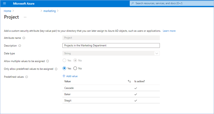
Step 1: Define attributes in Azure AD
The first step is to create an attribute set, which is a collection of related attributes. For example, you can create an attribute set called “marketing” to refer to the attributes related to the marketing department. The second step is to define the attributes inside the attribute set and the characteristics of the attribute set. For example, only pre-defined values are allowed for an attribute and whether an attribute can be assigned a single value or multiple values. In this example, there are three values for the project attribute—Cascade, Baker, and Skagit—and a user can be assigned only one of the three values. The picture below illustrates the above example.
Step 2: Assign attributes to users or enterprise applications
Once attributes are defined, they can be assigned to users, enterprise applications, and Azure managed identities.

Once you assign attributes, users or applications can be filtered using attributes. For example, you can query all enterprise applications with a sensitivity level equal to high.

Step 3: Delegate attribute management
There are four Azure AD built-in roles that are available to manage attributes.

By default, Global Administrators and Global Readers are not able to create, read, or update the attributes. Global Administrators or Privileged Role Administrators need to assign the attribute management roles to other users, or to themselves, to manage attributes. You can assign these four roles at the tenant or attribute set scope. Assigning the roles at tenant scope allows you to delegate the management of all attribute sets. Assigning the roles at the attribute set scope allows you to delegate the management of the specific attribute set. Let me explain with an example.

- Xia is a privileged role administrator; so, Xia assigns herself Attribute Definition Administrator role at the tenant level. This allows her to create attribute sets.
- In the engineering department, Alice is responsible for defining attributes and Chandra is responsible for assigning attributes. Xia creates the engineering attribute set, assigns Alice the Attribute Definition Administrator role and Chandra the Attribute Assignment Administrator role for the engineering attribute set; so that Alice and Chandra have the least privilege needed.
- In the marketing department, Bob is responsible for defining and assigning attributes. Xia creates the marketing attribute set and assigns the Attribute Definition Administrator and Attribute Assignment Administrator roles to Bob.
Step 4: Achieve fine-grained access control with fewer Azure role assignments
Let’s build on our fictional example from the previous blog post on ABAC conditions in Azure Role Assignments. Bob is an Azure subscription owner for the sales team at Contoso Corporation, a home improvement chain that sells items across lighting, appliances, and thousands of other categories. Daily sales reports across these categories are stored in an Azure storage container for that day (2021-03-24, for example); so, the central finance team members can more easily access the reports. Charlie is the sales manager for the lighting category and needs to be able to read the sales reports for the lighting category in any storage container, but not other categories.
With resource attributes (for example, blob index tags) alone, Bob needs to create one role assignment for Charlie and add a condition to restrict read access to blobs with a blob index tag “category = lighting”. Bob needs to create as many role assignments as there are users like Charlie. With user attributes along with resource attributes, Bob can create one role assignment, with all users in an Azure AD group, and add an ABAC condition that requires a user’s category attribute value to match the blob’s category tag value. Xia, Azure AD Admin, creates an attribute set “contosocentralfinance” and assigns Bob the Azure AD Attribute Definition Administrator and Attribute Assignment Administrator roles for the attribute set; giving Bob the least privilege he needs to do his job. The picture below illustrates the scenario.

Bob writes the following condition in ABAC condition builder using user and resource attributes:

To summarize, user attributes, resource attributes, and ABAC conditions allow you to manage access to millions of Azure storage blobs with as few as one role assignment!
Auditing and tools
Since attributes can contain sensitive information and allow or deny access, activity related to defining, assigning, and unassigning attributes is recorded in Azure AD Audit logs. You can use PowerShell or Microsoft Graph APIs in addition to the portal to manage and automate tasks related to attributes. You can use Azure CLI, PowerShell, or Azure Resource Manager templates and Azure REST APIs to manage ABAC conditions in Azure Role Assignments.
Resources
We have several examples with sample conditions to help you get started. The Contoso corporation example demonstrates how ABAC conditions can scale access control for scenarios related to Azure storage blobs. You can read the Azure AD docs, how-to’s, and troubleshooting guides to get started.
We look forward to hearing your feedback on Azure AD custom security attributes and ABAC conditions for Azure storage. Stay tuned to this blog to learn about how you can use custom security attributes in Azure AD Conditional Access. We welcome your input and ideas for future scenarios.
Learn more about Microsoft identity:
by Contributed | Nov 29, 2021 | Technology
This article is contributed. See the original author and article here.
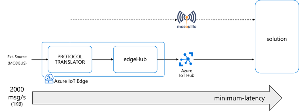
I had a customer streaming messages at a high-rate (up to 2000 msg/s – 1KB each) from a protocol translator running on an x86 industrial PC to a cloud-based Mosquito MQTT broker.
That edge device evolved quickly into a more capable and secure intelligent edge solution thanks to Azure IoT Edge and Azure IoT Hub, adding device provisioning (secured with an HW-based identity) and device management capabilities on top of a bi-directional communication, along with the deployment, execution, and monitoring of other edge workloads in addition to a containerized version of the original MQTT protocol translator.
The performance requirement did not change though: the protocol translator (running now as an Azure IoT Edge module) still had to ingest and deliver to the IoT Hub up to 2000 msg/s (1KB each), with a minimum latency.
Is it feasible? Can an IoT Edge solution stream 2000 msg/s or even higher rates? What’s the upper limit? How to minimize the latency?
This blog post will guide you through a detailed analysis of the pitfalls and bottlenecks when dealing with high-rate streams, to eventually show you how to optimize your IoT Edge solution and meet and exceed your performance requirements in terms of rate, throughput, and latency.
Topics covered:
The message queue
The Azure IoT Edge runtime includes a module named edgeHub, acting as a local proxy for the IoT Hub and as a message broker for the connected devices and modules.
The edgeHub supports extended offline operation: if the connection to the IoT Hub is lost, edgeHub saves messages and twin updates in a local message queue (aka “store&forward” queue). Once the connection is re-established, it synchronizes all the data with the IoT Hub.
The environment variable “UsePersistentStorage” controls whether the message queue is:
- stored in-memory (UsePersistentStorage=false)
- persisted on disk (UsePersistentStorage=true, which is the default


When persisted on disk (default), the location of the queue will be:
- the path you specified in the edgeHub HostConfig options in the deployment manifest as per here
- …or in the Docker’s OVERLAY folder if you didn’t do any explicit bind, which is:
/var/lib/docker/overlay2
The size of the queue is not capped, and it will grow as long as the device has storage capacity.
When dealing with a high message rate over a long period, the queue size could easily exceed the available storage capacity and cause the OS crash.
How to prevent the OS crash?
Binding the edgeHub folder to a dedicated partition, or even a dedicated disk if available, would protect the OS from uncontrolled growth of the edgeHub queue.

If the “DATA” partition (or disk) runs out of space:
- the OS won’t crash…
- …but edgeHub container will crash anyways!
How to prevent the edgeHub crash?
Do size the partition for the worst-case or reduce the Time-To-Live (TTL).
I will let you judge what’s the worst case in your scenario. But the very worst case is total disconnection for the entire TTL. During the TTL (which is 7200 s = 2 hrs. by default), the queue will accumulate all the incoming messages at a given rate and size. And be aware that the edgeHub keeps one queue per endpoint and per priority.
An estimation of the queue size on disk would be:

And if you do the math, a “high” rate of 2000 [msg/s] with 1 [KB/msg] could easily consume almost 15 GBs of storage within 2 hrs.

But even a “low” 100 [msg/s] rate you could easily consume up to 1GB, which would be an issue on constrained devices with an embedded storage of few GBs.

Then, to keep the disk consumption under control:
- the application requirements and what the “worst case” means in your scenario
- do some simple math to estimate the max size consumed by the edgeHub queue and size the partition/disk accordingly…
- …and fine-tune the TTL
If you keep the queue disk consumption under control with proper estimation and sizing, you don’t need to bind it to a dedicated partition/disk. But it’s an extra-precaution that comes with almost no effort.
Btw: If you considered setting UsePersistentStorage=false to store the queue in memory, you may realize now that the amount of RAM needed would make it an expensive option if compared to disk or non-viable at all. Moreover, such an in-memory store would NOT be resilient to unexpected crashes or reboots (as the “EnableNonPersistentStorageBackup” can backup and restore the in-memory queue only when you go through a graceful shutdown and reboot).

The clean-up process
What happens to expired messages?
Expired messages are removed every 30 minutes by default, but you can tune that interval using this environment variable MessageCleanupIntervalSecs:

If you use different priorities (LINK), do set “CheckEntireQueueOnCleanup”=true to force a deep clean-up and make sure that all expired messages are removed, regardless of the priority.

Why? The edgeHub keeps one queue per endpoint and per priority (but not per TTL)
If you have 2 routes with the same endpoint and priority but different TTL, those messages will be put in the same queue. In that case, it is possible that the messages with different TTLs are interleaved in that queue. When the cleanup processor runs, by default, it checks the messages on the head of each queue to see if they are expired. It does not check the entire queue, to keep the cleanup process as light as possible. If you want it to clean up all messages with an expired TTL, you can set the flag CheckEntireQueueOnCleanup to true.
The built-in metrics
Now that you have the disk consumption of your edgeHub queue under control, it’s a good practice to keep it monitored using the edgeAgent and edgeHub built-in metrics and the Azure Monitor integration.

The “edgeAgent_available_disk_space_bytes” reports the amount of space left on the disk.
…but there’s another metric you should pay attention to, which is counting the number of non-expired messages still in the queue (i.e. not delivered yet to the destination endpoint):
That “edgehub_queue_length” is a revelation, and it explains how the latency relates to the rates. But to understand it, we must measure the message rate along the pipeline first.
The analysis
How to measure the rates and the queue length
I developed IotEdgePerf, a simple framework including:
- a transmitter edge module (1), to be deployed on the edge device under test. It will generate a burst of messages and measure the actual output rate (at “A”)
- an ASA query (2), to measure the IoT Hub ingress rate (at “B”) and the end-2-end latency (“A” to “B”)
- a console app (3), to coordinate the entire test, to collect the results from the ASA job and show the stats
Further instructions in the IotEdgePerf GitHub repo.

I deployed the IotEdgePerf transmitter module to an IoT Edge 1.2 (instructions here) running on a DS2-v2 VM and connected to a 1xS3 IoT Hub. I launched the test from the console app as follows:
dotnet run --
--payload-length=1024
--burst-length=50000
--target-rate=2000
Here are the results:

- actual transmitter output rate (at “A”): 1169 msg/s, against the desired 2000 msg/s
- IoT Hub ingestion rate: 591 msg/s (at “B”)
- latency: 42s (“C”)
As anticipated, the “edgehub_queue_length” explains why we have the latency. Let’s have a look at it using Log Analytics:

Let’s correlate the queue length with the transmission burst: as the queue is a FIFO (First-In-First-Out), the last message produced by the transmitter is the last message ingested by the IoT Hub. Looking at “edgehub_queue_length” data, the latency on the last message is 42 seconds.

How does the queue’s growth and degrowth slopes and maximum value relate to the message rate?

- first, during the burst transmission, the queue grows with a rate:

which is in line with what you would expect from a queue, where the growth rate:

- then, once the transmission is over, the queue decreases with a rate:

The consistency among the different measurements (on the message rate, queue growth/degrowth and latency) proves that the methodology and tools are correct.
Minimum latency
Using some simple math, we can express the latency as:


where N is the number of messages.
If we apply that equation to the numbers we measured, again we can get a perfect match:


The latency will be minimum when rateOUT = rateIN, i.e. when the upstream rate equals the source output rate, and the queue does not accumulate messages. This is quite an obvious outcome, but now you have a methodology and tools to measure and relate to each other the rates, the latency, and the queue length (and the disk consumption as well).
Looking for bottlenecks
Let’s go back to the original goal of a sustained 2000 msg/s rate delivered upstream with minimum latency. We are now able to measure both the source output and the upstream rate, and to tell what’s the performance gap we must fill to assure minimum latency:
- the source output rate should increase from 1160 to 2000 msg/s (A)
- the upstream rate should increase from 591 to 2000 msg/s (B)

But… how to fill that gap? What’s the bottleneck? Do I need a faster CPU or more cores? More RAM? Or the networking is the bottleneck? Or are we hitting some throttling limits on the IoT Hub?
Scaling UP the hardware
Let’s try with a more “powerful” hardware.
Even if IoT Edge will usually run on a physical HW, let’s use IoT Edge on an Azure VMs, which provide a convenient way of testing different sizes in a repeatable way and compare the results consistently.
I measured the baseline performance of the DSx v2 VMs (general purpose with premium storage) sending 300K messages 1KB each using IotEdgePerf:
VM SIZE
|
SPECS (vCPU/RAM/SCORE)
|
Source
[msg/s]
|
Upstream
[msg/s]
|
Standard_DS1_v2
|
1 vcpu / 3.5 GB / ~20
|
900 ÷ 1300
|
500 ÷ 600
|
Standard_DS2_v2
|
2 vcpu / 7 GB / ~40
|
Standard_DS3_v2
|
4 vcpu / 7 GB / ~75
|
Standard_DS4_v2
|
8 vcpu / 14 GB / ~140
|
Standard_DS5_v2
|
16 vcpu / 56 GB / ~300
|
(test conditions: 1xS3 IoT Hub unit, this C# transmitter module, 300K msg, msg size 1KB)
Scaling UP from DS1 to DS5, the source rate increases by around ~50% from a DS1 to DS5… which is peanuts if we consider that a DS5 performs ~15x better (scores here) and costs ~16x (prices here) than a DS1.
Even more interestingly, the upstream rate does not increase, suggesting there’s a weak correlation (or no correlation at all) with the HW specs.
Scaling OUT the source
Let’s distribute the source stream across multiple modules in a kind of scaling OUT, and look at the aggregated rate produced by all the modules.


The maximum aggregated source is ~1900 msg/s rate (obtained with N=3 modules), which is higher than the rate of a single module (~1260 msg/s), with a gain of ~50%. However, such improvement is not worth it if we consider the higher complexity of distributing the source stream across multiple source modules.
Interestingly, the upstream rate increases from ~600 to ~1436 msg/s. Why?
The edgeHub can either use the AMQP or the MQTT protocol to communicate upstream with the cloud, independently from protocols used by downstream devices. The AMQP protocol provides multiplexing capabilities that allow the edgeHub for combining multiple downstream logical connections (i.e. the many modules) into a single upstream connection, which is more efficient and leads to the rate improvement that we measured. AMQP is indeed the default upstream protocol and the one I used in this test. This also confirms that the upstream rate is mostly determined by the protocol stack overhead.
Many cores with many modules
Scaling UP from a 1 vCPU machine (DS1) to a 16 vCPU (DS5) machine didn’t help when using a single source module. But what if we have multiple source modules? Would many cores bring an advantage?

Yes. Multiple modules mean multiple docker containers and eventually multiple processes, that will run more efficiently on a multi-core machine.
But is the 3.5x boost worth the 16x price increase of a DS5 vs DS1? No, if you consider that the upstream, again, didn’t increase.
Increasing the message size: from rate to throughput
Let’s go back to a single module and increase the message size from 1 KB to 32 KB on a DS1v2 (1 vcpu, 3.5GB). Here are the results:

(test conditions: 1xS3 IoT Hub unit, this C# transmitter module)
The rate decreases from 839msg/s@1KB down to 227msg/s@32KB, but the THROUGHPUT increases from ~0.8 MB/s up to ~7.2MB/s. Such behavior suggests that sending big messages and at a lower rate is more efficient!
How to leverage it?
Let’s assume that the big 16KB message is a batch of 16 x 1 KB messages: it means that the ~4.5MB/s throughput would be equivalent to a message rate of ~4500 msg/s of 1KB each.
Then message rate and throughput is not the same thing. If the transport protocol (and networking) is the bottleneck, higher throughputs can be achieved by sending bigger messages at a lower rate.
How do we implement message batching then?
Message Batching
We have two options:
- Application-level batching: the batching is done in the source module, whereas the downstream service extracts the original individual messages. This requires custom logic at both ends.

- edgeHub built-in batching: the batching is managed by the edgeHub and the IoT Hub automatically and in a transparent way, without the need for any additional code.
The ENV variable “MaxUpstreamBatchSize” sets the max number of messages EdgeHub will batch together into a single message up to 256KB.

edgeHub built-in batching deep dive
The default is MaxUpstreamBatchSize = 10, meaning that some batching is already happening under the cover, even if you didn’t realize it. The optimal value for MaxUpstreamBatchSize would be 256 KB / size(msg), as you would want to fit as many small messages as you can in the batch message.
How does it work?
Set the edgeHub RuntimeLogLevel to DEBUG and look for lines containing “obtained next batch for endpoint iothub”:

Looking at the timestamps, you’ll see that messages are collected and sent upstream in a batch every 20ms, suggesting that:
- the latency introduced by this built-in batching is negligible (< 20ms)
- this mechanism is effective only when the input rate is > 1/20ms=50 msg/s
Comparison of the batching options
Are the application-level and built-in batching equivalent?

On the UPSTREAM side, you have batch messages (i.e. big and low-rate) in both cases. It means that:
- you pay for the batch size divided by 4KB
- and the batch messages counts as a single d2c operation
The latter point is quite interesting: as the message batch counts as 1 device-to-cloud operation, the batching helps also reduce the pressure on the d2c throttling limit of the IoT Hub, which is an attention point when dealing with high message rates.

On the SOURCE side, the two approaches are very different:
- application-level batching is sending batch messages (i.e. big, and low-rate)
- …while the built-in batching is sending the individual high-rate small messages, and potentially still less efficient (think of the IOPS on the disk for instance, and the transport protocol used to publish the messages to the edgeHub broker).
Eventually, we can state that:
- application-level batching is efficient end-2-end (i.e. source and upstream)…
- …while the built-in batching is efficient on the upstream only
Let’s test that assumption.
Built-in batching performance
On a DS2v2 VM, the max output rate of the source module is ~1100 [msg/s] (with 1KB messages).
As expected, such source rate does not benefit from higher MaxUpstreamBatchSize values, while the upstream does, and it eventually equals the 1100 [msg/s] source rate (hence no latency).


Application-level batching performance
The application-level batching is effective on both the source and upstream throughput.

On a DS1 (1 vCPU, 3.5GB of RAM, which is the smallest size of the DSv2 family) you can achieve:
- a sustained ~3600 [KB/s] end-to-end with no latency (i.e. on both source and upstream) with a msg size of 8KB…
- …while with a msg size of 32KB, you can increase the source throughput up to 7300 [KB/s], but the upstream is capped at around 4200 KB/s. That will cause some latency.


Is latency always a problem? Not actually. As we saw, the latency is proportional to the number of messages sent (N):

When sending a short burst of messages, the latency may be negligible. On the other hand, on short burst you may want to minimize the transmission duration.
As an example, let’s assume you want to send N=1000 messages, of 1 KB each. Depending on the batching, the transmission duration at the source side will be:
- no batching: transmission duration = 1000 / 872 ~ 1.1s (with no latency)
- 8KB batching: transmission duration = 1000 / 3648 ~ 0.3s (with no latency)
- 32KB batching: transmission duration = 1000 / 7328 ~ 0.1s (+0.2s of latency)
Shortening the transmission duration from a 1.1s down to 0.1s could be critical in battery powered applications, or when the device must send some information upon an unexpected loss of power.
Azure IoT Device SDKs performance comparison
The performance results discussed in this blog post were obtained using this C# module, which leverages the .NET Azure IoT Device SDK.
How do other SDKs (Python, Node.js, Java, C) perform in terms of maximum message rate and throughput? The performance gap, if any, would be due to:
- language performance (C is compiled whereas others are interpreted)
- specific SDK architecture and implementation
As an example of the latter, the JAVA SDK differs from other SDKs as the device/module client embeds a queue and a periodic thread that checks for queued messages. Both the thread period (“receivePeriodInMilliseconds”) and the number of messages de-queued per execution (“SetMaxMessagesSentPerThread”) can be tweaked to increase the output rate.
On the other hand, what is the common denominator to all the SDKs? It’s the transport protocol, which ultimately sets the upper bound of the achievable performance. In this blog post we focused on MQTT, and it would be worth to explore the performance upper bound by using a fast and lightweight MQTT client instead of the SDK. That’s doable and it’s explained here.
A performance comparison among the different Device SDKs as well as a MQTT client will be the topic for a next blog post.
Tools
VM provisioning script
A bash script to spin up a VM with Ubuntu Server 18.04 and a fully provisioned Azure IoT Edge ready-to-go: https://github.com/arlotito/vm-iotedge-provision

IotEdgePerf
A framework and a CLI tool to measure the rate, the throughput and end-to-end latency of an Azure IoT Edge device:
https://github.com/arlotito/IotEdgePerf


Conclusion
This blog post provided a detailed analysis of the pitfalls and bottlenecks when dealing with high-rate streams, and showed you how to optimize your IoT Edge solution to meet and exceed your performance requirements in terms of rate, throughput, and latency.
On an Azure DS1v2 Virtual Machine, we were able to meet and exceed the original performance target of 2000 msg/s (1KB each) and minimum latency, and we achieved a sustained end-2-end throughput of 3600 KB/s with no latency, or up to 7300 msg/s (1KB each) with some latency.
With the methodology and tools discussed in this blog post, you can assess the performance baseline on your specific platform and eventually optimize it using the built-in or application-level message batching.
In a nutshell:
- to avoid the OS and edgeHub crash:
- do estimate the maximum queue length and do size the partition/disk accordingly
- adjust the TTL
- keep the queue monitored using the built-in metrics
- measure the baseline performance (rate, throughput, latency) of your platform (using IotEdgePerf) and identify the bottlenecks (source module? Upstream?)
- if the bottleneck is the upstream, leverage the built-in batching by tuning the MaxUpstreamBatchSize
- if the bottleneck is the source module, use application level-batching
- possibly try a different SDK or a low-level MQTT client for maximum performance
Acknowledgements
Special thanks to the Azure IoT Edge team (Venkat Yalla and Varun Puranik), the Industry Solutions team (Simone Banchieri, Stefano Causarano and Franco Salmoiraghi), the IoT CSU (Vitaliy Slepakov and Michiel van Schaik) and Olivier Bloch for the support and the many inspiring conversations.


Recent Comments