by Scott Muniz | Jun 30, 2020 | Azure, Microsoft, Technology, Uncategorized
This article is contributed. See the original author and article here.
Azure APIM – Validate API requests through Client Certificate using Portal, C# code and Http Clients
Client certificates can be used to authenticate API requests made to APIs hosted using Azure APIM service. Detailed instructions for uploading client certificates to the portal can be found documented in the following article – https://docs.microsoft.com/en-us/azure/api-management/api-management-howto-mutual-certificates-for-clients
Steps to authenticate the request –
- Via Azure portal
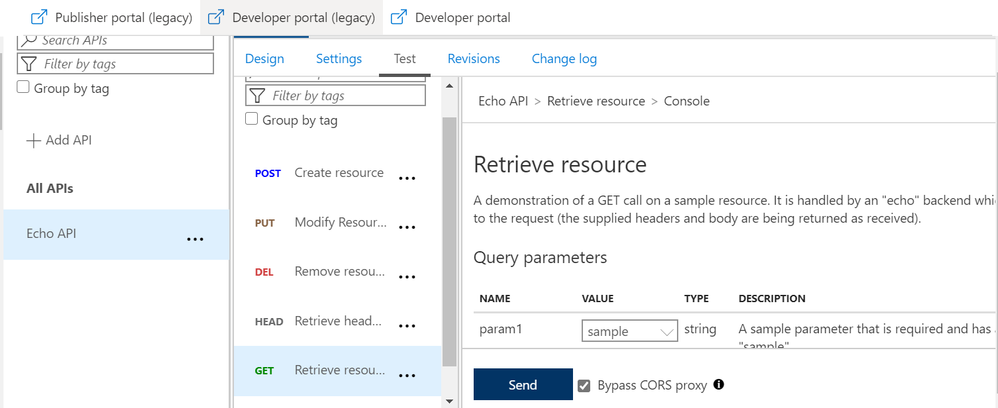
Once we have setup the certificate authentication using the above article, we can test an operation for a sample API (Echo API in this case). Here, we have chosen a GET operation and selected the “Bypass CORS proxy” option.
Once you click on the “Send” option, you would be asked to select the certificate that you would have already installed on your machine.

Note – This is the same certificate that you would have uploaded for your APIM service and added to the trusted list in the certificate store of your workstation.

After successful authentication and request processing, you would receive the 200 OK response code. Upon maneuvering to the trace logs, you can also see the certificate thumbprint that was passed for authentication.


The inbound policy definition used for this setup is as below:
(Kindly update the certificate thumbprint with your client certificate thumbprint)
<choose>
<when condition="@(context.Request.Certificate == null || context.Request.Certificate.Thumbprint != "BF3D644C46099A9D7C073EC002312878B8F9B847")">
<return-response>
<set-status code="403" reason="Invalid client certificate" />
</return-response>
</when>
</choose>
- Through C# or any other language that supports SDKs–
We can use the below sample C# code block to authenticate API calls and perform API operations.
Kindly update the below highlighted values with your custom values before executing the sample code attached below
Client certificate Thumbprint: BF3D644C46099A9D7C073EC002312878B8F9B847
Request URL: https://testapicert.azure-api.net/echo/resource?param1=sample
Ocp-Apim-Subscription-Key: 4916bbaf0ab943d9a61e0b6cc21364d2
Sample C# Code:
using System;
using System.IO;
using System.Net;
using System.Security.Cryptography.X509Certificates;

namespace CallRestAPIWithCert
{
    class Program
    {
        static void Main()
        {
            // EDIT THIS TO MATCH YOUR CLIENT CERTIFICATE: the subject key identifier in hexadecimal.
            string thumbprint = "BF3D644C46099A9D7C073EC002312878B8F9B847";
            X509Store store = new X509Store(StoreName.My, StoreLocation.CurrentUser);
            store.Open(OpenFlags.ReadOnly);
            X509Certificate2Collection certificates = store.Certificates.Find(X509FindType.FindByThumbprint, thumbprint, false);
            X509Certificate2 certificate = certificates[0];
            System.Net.ServicePointManager.SecurityProtocol = SecurityProtocolType.Tls12;
            ServicePointManager.ServerCertificateValidationCallback = new System.Net.Security.RemoteCertificateValidationCallback(AcceptAllCertifications);

            HttpWebRequest req = (HttpWebRequest)WebRequest.Create("https://testapicert.azure-api.net/echo/resource?param1=sample");
            req.ClientCertificates.Add(certificate);
            req.Method = WebRequestMethods.Http.Get;
            req.Headers.Add("Ocp-Apim-Subscription-Key", "4916bbaf0ab943d9a61e0b6cc21364d2");
            req.Headers.Add("Ocp-Apim-Trace", "true");
            Console.WriteLine(Program.CallAPIEmployee(req).ToString());
            Console.WriteLine(certificates[0].ToString());

            Console.Read();

        }

        public static string CallAPIEmployee(HttpWebRequest req)
        {
            var httpResponse = (HttpWebResponse)req.GetResponse();
            using (var streamReader = new StreamReader(httpResponse.GetResponseStream()))
            {
                return streamReader.ReadToEnd();
            }
        }

        public static bool AcceptAllCertifications(object sender, X509Certificate certification, X509Chain chain, System.Net.Security.SslPolicyErrors sslPolicyErrors)
        {
            return true;
        }
    }
}
- Through Postman or any other Http Client
To use client certificate for authentication, the certificate has to be added under PostMan first.
Maneuver to Settings >> Certificates option on PostMan and configure the below values:
Host: testapicert.azure-api.net (## Host name of your Request API)
PFX file: C:UserspraskumaDownloadsabc.pfx (## Upload the same client certificate that was uploaded to APIM instance)
Passphrase: (## Password of the client certificate)

Once the certificate is uploaded on PostMan, you can go ahead and invoke the API operation.
You need to add the Request URL in the address bar and also add the below 2 mandatory headers:
Ocp-Apim-Subscription-Key : 4916bbaf0a43d9a61e0bsssccc21364d2 (##Add your subscription key)
Ocp-Apim-Trace : true
Once updated, you can send the API request and receive a 200 OK response upon successful authentication and request processing.

For detailed trace logs, you can check the value for the output header – Ocp-Apim-Trace-Location and retrieve the trace logs from the generated URL.

by Scott Muniz | Jun 30, 2020 | Azure, Microsoft, Technology, Uncategorized
This article is contributed. See the original author and article here.
Azure Migrate now supports assessments for Azure VMware Solution, providing even more options for you to plan your migration to Azure. Azure VMware Solution (AVS) enables you to run VMware natively on Azure. AVS provides a dedicated Software Defined Data Center (SDDC) for your VMware environment on Azure, ensuring you can leverage familiar VMware tools and investments, while modernizing applications overtime with integration to Azure native services. Delivered and operated as a service, your private cloud environment provides all compute, networking, storage, and software required to extend and migrate your on-premises VMware environments to the Azure.
Previously, Azure Migrate tooling provided support for migrating Windows and Linux servers to Azure Virtual Machines, as well as support for database, web application, and virtual desktop scenarios. Now, you can use the migration hub to assess machines for migrating to AVS as well.
With the Azure Migrate: Server Assessment tool, you can analyze readiness, Azure suitability, cost planning, performance-based rightsizing, and application dependencies for migrating to AVS. The AVS assessment feature is currently available in public preview.
This expanded support allows you to get an even more comprehensive assessment of your datacenter. Compare cloud costs between Azure native VMs and AVS to make the best migration decisions for your business. Azure Migrate acts as an intelligent hub, gathering insights throughout the assessment to make suggestions – including tooling recommendations for migrating VM or VMware workloads.
How to Perform an AVS Assessment
You can use all the existing assessment features that Azure Migrate offers for Azure Virtual Machines to perform an AVS assessment. Plan your migration to Azure VMware Solution (AVS) with up to 35K VMware servers in one Azure Migrate project.
- Discovery: Use the Azure Migrate: Server Assessment tool to perform a datacenter discovery, either by downloading the Azure Migrate appliance or by importing inventory data through a CSV upload. You can read more about the import feature here.
- Group servers: Create groups of servers from the list of machines discovered. Here, you can select whether you’re creating a group for an Azure Virtual Machine assessment or AVS assessment. Application dependency analysis features allow you to refine groups based on connections between applications.
- Assessment properties: You can customize the AVS assessments by changing the properties and recomputing the assessment. Select a target location, node type, and RAID level – there are currently three locations available, including East US, West Europe and West US, and more will continue to be added as additional nodes are released.
- Suitability analysis: The assessment gives you a few options for sizing nodes in Azure, between performance-based or as on-premises. It checks AVS support for each of the discovered servers and determines if the server can be migrated as-is to AVS. If there are any issues found, the assessment automatically provides remediation guidance.
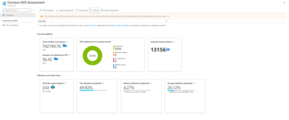
- Assessment and cost planning report: Run the assessment to get a look into how many machines are in use and what estimated monthly and per-machine costs will be in AVS. The assessment also recommends a tool for migrating the machines to AVS. With this, you have all the information you need to plan and execute your AVS migration as efficiently as possible.

Figure 1 Assessment and Cost Planning Report

Figure 2 AVS Readiness report with suggested migration tool
Learn More
by Scott Muniz | Jun 30, 2020 | Azure, Microsoft, Technology, Uncategorized
This article is contributed. See the original author and article here.
1. Install .NET Core 3
Azure Functions v3 runs on .NET Core 3.
To install .NET Core 3, visit Download .NET Core.
I recommend selecting the latest LTS version. LTS stands for Long Term Support, meaning that Microsoft is committed to supporting this specific version of .NET Core with bug fixes for approximately 2-3 years.
As of today, the current LTS version of .NET Core is .NET Core 3.1.
2. Update the CSPROJ
Let’s ensure our csproj file has been updated for Azure Functions v3.
We’ll need to set the following three things:
Here is an example from my GitTrends app: https://github.com/brminnick/GitTrends/blob/master/GitTrends.Functions/GitTrends.Functions.csproj
<?xml version="1.0" encoding="utf-8"?>
<Project Sdk="Microsoft.NET.Sdk">
    <PropertyGroup>
        <TargetFramework>netcoreapp3.1</TargetFramework>
        <AzureFunctionsVersion>v3</AzureFunctionsVersion>
    </PropertyGroup>
    <ItemGroup>
        <PackageReference Include="Microsoft.NET.Sdk.Functions" Version="3.0.1" />
    </ItemGroup>
    <ItemGroup>
        <None Update="host.json">
            <CopyToOutputDirectory>PreserveNewest</CopyToOutputDirectory>
        </None>
        <None Update="local.settings.json">
            <CopyToOutputDirectory>PreserveNewest</CopyToOutputDirectory>
            <CopyToPublishDirectory>Never</CopyToPublishDirectory>
        </None>
    </ItemGroup>
</Project>
3a. (Visual Studio) Update Azure Functions Runtime
Note: If you’re using Visual Studio for Mac, skip to the next section
Let’s now install the Azure Functions Runtime for Visual Studio 2019
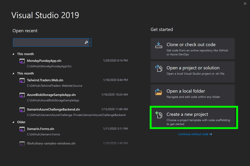
- In Visual Studio, select Create a new project
 Visual Studio, Create New Project
2. In the Create a new project window, in the search bar, enter Functions
3. In the Create a new project window, in the search results, select Azure Functions
4. In the Create a new project window, select Next
 Create a new Azure Functions Project
5. In the Create a new Azure Functions Application window, stand by while it is “Getting information about the latest function tools…”

6. In the Create a new Azure Functions Application window, once the new tools have been downloaded, click Refresh

3b. (Visual Studio for Mac) Update Azure Functions Runtime
Note: If you are using Visual Studio on PC, you may skip this step
Let’s now install the Azure Functions Runtime for Visual Studio for Mac
- In the Visual Studio for Mac window, select New
2. In the New Project window, on the left-hand menu, under Cloud, select General
3. In the Configure you Azure Functions Project window, standby until it finishes installing the Azure Functions components
 Update Functions Runtime
4. Conclusion
Updating to Azure Functions v3 requires a couple steps:
- Installing .NET Core 3
- Updating our csproj
- Updating Visual Studio’s Azure Functions Runtime
If you’d like to see an existing Azure Functions project using v3, feel free to check the Azure Functions Backend in my GitTrends app: https://github.com/brminnick/GitTrends/tree/master/GitTrends.Functions
by Scott Muniz | Jun 30, 2020 | Azure, Microsoft, Technology, Uncategorized
This article is contributed. See the original author and article here.
We often hear that customers need help determining the best option when migrating their on-premises SQL Server to Azure. See the link below to the blog and video we developed to address that question. The video will help you begin your migration journey to Azure SQL by learning about the best options available for SQL Server migration to Azure based on your unique needs.
https://techcommunity.microsoft.com/t5/azure-migration/sql-server-best-options-for-database-migration-into-azure/ba-p/1497339
by Scott Muniz | Jun 30, 2020 | Azure, Microsoft, Technology, Uncategorized
This article is contributed. See the original author and article here.
Organizations are increasingly looking to migrate their on-premises databases to cloud, whether to take advantage of built-in high availability and disaster recovery features or to reduce operating costs by getting rid of administrative overhead and becoming more efficient. While customers recognize the benefits of moving to the cloud, they need help and guidance on planning and executing migration of their databases.
We often hear that customers need help determining the best option when migrating their on-premises SQL Server to Azure. We developed this video to address that question. The video will help you begin your migration journey to Azure SQL by learning about the best options available for SQL Server migration to Azure based on your unique needs. From simple ‘lift-and-shift’ migrations to an Azure virtual machine (VM), to modernization to fully managed database-as-a-service, you can leverage this guidance to quickly move your databases. See how to realize cost savings and efficiencies with offers like Azure Hybrid Benefit and free Extended Security Updates. You’ll watch an online migration performed starting with an assessment of databases and applications using Azure Migrate and completing the migration process with Azure Database Migration Service (DMS). See how easily you can translate your existing SQL Server knowledge to perform the migration yourself!
For advice on what Azure SQL destination to use for your workload, try our Choose Your Database tool.
To learn more about migrating SQL Server to Azure, check out the learning paths and modules available on MS Learn or take a look at the Azure Database Migration Guide.
by Scott Muniz | Jun 29, 2020 | Azure, Microsoft, Technology, Uncategorized
This article is contributed. See the original author and article here.
Introduction
In this article, we’re going to talk about enabling MFA for applications that are accessed over the internet. This will force users accessing the application from the internet to authenticate with their primary credentials as well as a secondary using Azure MFA.
Enabling App Service Authentication for a Web App
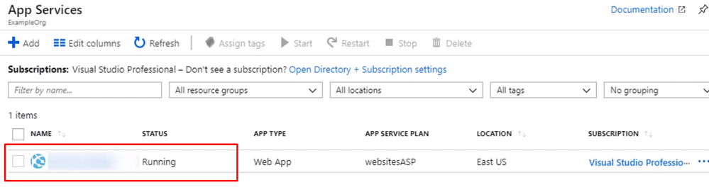
In this guide step by step, I’m going to show you how to enable MFA for an Azure App Service web app so authentication is taken care of by Azure Active Directory, and users accessing the app are forced to perform multifactor authentication using conditional access policy that Azure AD will enforce. To set up the environment, We will assume there is an Azure web app that is deployed to Azure Portal

Open up the management blade for this app service, and let’s scroll down to Authentication/Authorization. This allows us to add authentication for users accessing the app

Enable the App Service Authentication and Action to login with Active directory and then click Activity Directory option to configure

Select the express settings, and this will create an app registration in Azure Active Directory. The registration creates a service principle that represent the application and enables the functionality to grant it access to other Azure resources this will be using the app registration later when we create a conditional access policy to enforce Azure MFA. Click OK to enable this and save the changes.


Testing the app. Open a new browser and browse to the application address. You should be redirected to the Azure AD Login page to sign-in using your Azure AD credentials due enabling App Service Authentication.


Configuring MFA for an App Service Web App
We’ve got a working App Service web app with authentication set to redirect the user to log in with their Azure Active Directory credentials. Now let’s create a conditional access policy that forces the user to use Azure MFA for this particular app.
From the Active Directory blade, Scroll down to the Conditional Access menu

Give the policy a name for the interface and select Users and groups, and I want this policy to apply to anyone accessing the application, but you could scope it to a particular Azure AD group, user, or a directory role.
Select the app that this policy will apply to, and we want to choose the app registration that was created for our App Service web app when we enabled authentication and authorization. So that’s called appformfa. Click Done.


Go to Access controls, and it’s set to grand access. Select require multifactor authentication, that. And don’t forget to enable the policy and click Create. The policy is now enabled for the App Service.


Open up a new browser window, and navigate to the App Service web app URL, Log in with the same user as before.


If this user wasn’t set up, they’d be prompted to set up MFA. The conditional access policy for the app is now requiring that the user log in with Azure MFA.
Enter the one-time passcode into the browser, and you will be brought into the app.


That is, we successfully enabled MFA for Azure web app.
Thank you
Magdy Salem
Credit: The blog was inspired by Pluralsight course Azure MFA Implementation

Recent Comments