This article is contributed. See the original author and article here.
The COVID-19 pandemic has pushed “order management” from the backend of logistics operations to the spotlight of supply chain and commerce strategies. Retailers, consumer package goods (CPG) companies, and distributors rushed to adapt their business models to fulfill the explosive growth of online orders through different digital channels. End-customers and organizations buy through various channels such as marketplaces, in-store, mobile apps, and even social media. They expect faster and more convenient ways for pickups and returns, such as pickup in-store, at a partner’s location, and for returns, drop off at the nearest location, QR codes, and even at-home pickup.
As the number of order sources and fulfillment options grow exponentially, organizations need the right order management solution to keep up with the evolving digital commerce landscape. This blog looks at three key aspects to consider when selecting an order management solution and how Microsoft Dynamics 365 Intelligent Order Management can help you.
1. Open and modern platform
The adoption of online shopping, and the addition of more consumers and businesses online for all types of transactions with the pandemic, have created a demand for convenience and personalization in digital commerce. As the number of online marketplaces grows, retailers, CPG, distributors, and manufacturers with business-to-business (B2B) and direct-to-consumer (D2C) business models require to accept orders from an ever-growing external ecosystem. Receiving orders from multiple sources increases order management and supply chain complexity. Therefore, these organizations need an order management solution that helps them accept orders from anywhere to keep pace with the continuing evolution of e-commerce.
Dynamics 365 Intelligent Order Management has an open and modern platform that seamlessly integrates with organizations’ existing tech stack. Its architecture reduces implementation time through out-of-the-box pre-built connectors to the best-of-breed ecosystem of partners for order source, delivery, tax compliance, price calculation, and logistics services such as Adobe Commerce, J.B. Hunt, Krber, Uber Freight, Avalara, Vertex, Flexe, Big Commerce, Far Eye, Commerce Tools, Flintfox, Ship Station, and Orderful. Moreover, this platform architecture is composable and flexible to allow supply chain professionals to build in an incremental way through a modular and API-first approach and a supply chain control tower, which ultimate goal is supply chain visibility.
2. Real-time visibility and intelligent fulfillment optimization
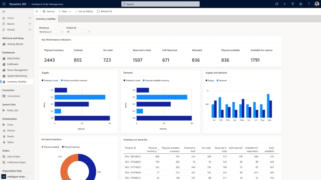
The 2021 Gartner supply chain risk and resilience survey shows that for 83 percent of large organizations, better supply chain ecosystem visibility is a top priority.1 And another Gartner research shows that 60 percent of chief supply chain officers (CSCOs) are expected to make faster, more accurate, and consistent decisions in real-time.2 The cycle-time of business processes continues to accelerate, particularly in order management processes that serve consumers who expect faster and more convenient shipping to the location of their choice. To succeed in these conditions, companies need a solution that simplifies omnichannel order fulfillment by providing real-time visibility and AI-infused real-time data.
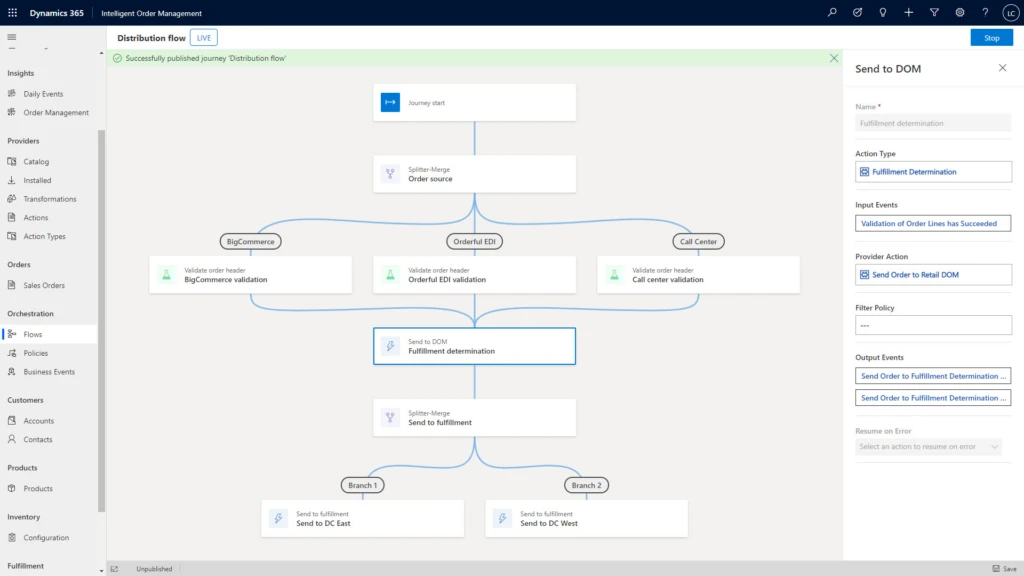
With Dynamics 365 Intelligent Order Management, supply chain and commerce professionals can model and automate responses to order constraints by using a journey orchestration designer and assigning rules in a low-code/no-code friendly user interface with drag and drop actions instead of coding. Dynamics 365 Intelligent Order Management uses an intelligent fulfillment optimization service to infuse AI into order fulfillment within your supply chain network. The intelligent optimization engine works to ensure the right products are delivered from the right source in the right quantities so that you always maximize profits, minimize costs, and satisfy service-level requirements.
3. Faster deployment times
Accepting orders from anywhere carries an additional challenge: implementation. Businesses need an order management solution that allows them to get up and running quickly. Not only do they need to be able to accept orders from anywhere, but many organizations also have existing systems that they would like to augment, not replace. If you are in the process of updating your order management system and fall into this category, then understanding what is involved in the implementation process is critically important. Will custom coding be required to integrate with your enterprise resource planning (ERP) and warehouse management system (WMS)? How about your customer relationship management (CRM) or transportation management system (TMS)? For most, the best solution is a cloud-based integrated-service-as-a-software (iSaaS) that uses RESTful APIs and can be easily configured using a low-code/no-code user interface.
Applications that take this approach enable supply chain and commerce professionals to continue to use and benefit from legacy applications, while also providing the agility to easily connect and integrate with modern web-based solutions. This is the approach that we have taken with Dynamics 365 Intelligent Order Management because it delivers these benefits and accelerates the digital transformation process regardless of where a company is in its digital transformation journey.
It is essential to look for an order management solution that will give you out-of-the-box pre-built connectors to an ecosystem of partners, provide real-time order visibility, intelligent fulfillment optimization, and get up you running quickly with seamless integration with your existing tech stacks, such as ERP and CRM systems. Traditional, on-premises order management systems can lack the flexibility required to keep pace with the rapidly evolving world of e-commerce.
With Dynamics 365 Intelligent Order Management, you can leverage our modern cloud technology, integrate with your existing platforms, and quickly implement new capabilities that enable AI, automation, order flow orchestration, and on-demand scalability. Get started today with Dynamics 365 Intelligent Order Management free trial and turn order fulfillment into a competitive advantage.
GARTNER is the registered trademark and service mark of Gartner Inc., and/or its affiliates in the U.S. and internationally and has been used herein with permission. All rights reserved.
This article is contributed. See the original author and article here.
Google has released Chrome version 99.0.4844.84 for Windows, Mac, and Linux. This version addresses a vulnerability that an attacker could exploit to take control of an affected system.
CISA encourages users and administrators to review the Chrome Release Note and apply the necessary updates.
This article is contributed. See the original author and article here.
From time to time we have users who open the same question multiple times.
The Issue – direct result of duplicate threads:
(1) Supporters – People that come to help might waste their time on something that was answered in the other thread.
(2) Users – people that search for the same issue might find the thread which has less information and miss the information in the other thread.
(3) original poster (OP) – the person who asked the question will probably not remember to follow all the threads which he opened.
Supporters and Users will waste time on responds which no one will read.
OP might miss the best answer/discussion while following a different thread.
In short, this is a lose-lose case where everyone lose!
Best practice for Moderators
In each interface the features which are built-in are different so these option might not fit all forums interfaces. With that said, as I want to focus mainly on the QnA forums, I will provide my insights according to the QnA features exists at this time.
The list is sorted from the best option for first time case – note that a user which continue such action is a different story. I the OP was inform on the issue and was asked to avoid such cases, then his behavior can be considered as abusive and should be treated accordingly.
In any case, the options which prevent such issue in advance, will be best!
Clear Policy document
In any communication interface, there must be a clear policy document which we can point the OP to. A link to the policy document must be presented in a way that no one will miss it and that everyone can view it from any page where the OP post his question. Usually it is recommended to add a clear link at the top of the page.
An intellisense feature
An intellisense feature provides information while the user type the content. It is well common in code editors in order to provide code completion, parameter info, quick info, and member lists. In the scope of the the discussion an intellisense feature will provide the user a list of previous thread according to the information he is typing.
Note! This feature existing at Microsoft QnA forums.
Insights!
Do not assume that the OP saw the forum policy or noticed the content of the intellisense information! Most people are focusing on their needs and ignore “background noises”. It may not be the most positive behavior but it is definitely a natural behavior.
Contact the OP in private
How?
If the system include an option to send internal private message then this is your best action!
The user email should be visible to other users, but if this information is available to you and there is no internal messaging feature, then send the user an email.
If there is no build-in messaging feature, then check the user profile and signature for links to his social media network (Facebook, Twitter, linkedin and so on) and send him a private message.
What?
Inform the user about the forum policy, add a link to the official policy document if exists and ask him to avoid such cases in the future. Don’t forget to send him links to all the duplicate threads which you found. Ask the user to select one of the threads, in all other thread add a link to the active thread and close the rest of the threads as duplicated.
Note! This feature not available to community moderators at Microsoft QnA forums.
Contact the OP in public
Add a response to the problematic message(s).
In most social media network a user which is not connected to you will not see your message. In this case you can add a response to one of the user last discussions. Remember that this is a public message and you should be extremally polite! Do not use this option if not must.
Provide the same information as in the case of private message
Note!
Taking actions behind the scenes has no value for the future behavior of the user and might lead the user to re-do the same, as he was not inform about an issue – this only raise the issue as it lead for more duplicate threads (actions behind the scene are for example deleting message, reporting message, and so on).
If you chose to take an action behind the scenes then you should also try to inform the OP about the taken actions!
Merge duplicate threads
By merging the duplicate threads you can ensure that no information is lost. Users who go to each of the links to the separate threads come to the same place – the merged thread. With that said, this action makes it a little difficult to orient in a discussion because one discussion combines responses from several discussions and the order of the messages can be confusing.
Note! This feature NOT existing at Microsoft QnA forums. It is exist in the MSDN forums.
Lock the duplicate thread(s) & comments
By locking the duplicate threads you can ensure that no information is lost. Users can still navigate to each of the links and watch the separate discussion. It is HIGHLY important to add a message that explain why this thread was locked and provide a link to the active thread.
In the QnA system locking the thread is done by closing the thread. It is important to know that close the thread does not prevent people from adding comments! You should go over each of the messages in the thread and lock the comment!
Note! This feature existing at Microsoft QnA forums.
Redirect the duplicate thread(s) to the one selected for continuing the discussion.
Redirecting users from a thread to another thread has a very problematic side effect: The original link still exists but it cannot be used to get the original message. This makes it harder to report the issue since the link redirect to an active thread and it make it impossible to inform the user about the issue and show him the duplicated thread.
Do not! (on the first case)
Do not treat the user as abuser! It can be a mistake.
Do not delete a message without informing the user. He might not find the message and create another new message.
Do not report the message without informing the user at the same time, since he cannot see the report and know about the issue.
Do you want to add your insights? You can add comments to this post or contact me in private if you want me to update the post, and in the meantime just remember to have fun and continue helping others.
This article is contributed. See the original author and article here.
Azure Data Factory and Azure Synapse Analytics introduced 2 exciting new features in mapping data flows recently that we have announced as generally available this week!
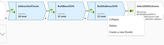
Flowlets: Create reusable portions of data flow logic that you can share in other pipelines as inline transformations. Flowlets enable ETL jobs to be composed of custom or common logic components.
Change Feed connectors are available in data flow source transformations for Cosmos DB, Blob store, ADLS Gen1, ADLS Gen2, and CDM. By simply checking the box shown below, you can tell ADF to manage a checkpoint automatically for you and only read the latest rows that were updated or inserted since the last pipeline run.
This article is contributed. See the original author and article here.
CISA has added 66 new vulnerabilities to its Known Exploited Vulnerabilities Catalog, based on evidence of active exploitation. These types of vulnerabilities are a frequent attack vector for malicious cyber actors and pose significant risk to the federal enterprise. Note: to view the newly added vulnerabilities in the catalog, click on the arrow on the of the “Date Added to Catalog” column, which will sort by descending dates.
Although BOD 22-01 only applies to FCEB agencies, CISA strongly urges all organizations to reduce their exposure to cyberattacks by prioritizing timely remediation of Catalog vulnerabilities as part of their vulnerability management practice. CISA will continue to add vulnerabilities to the Catalog that meet the specified criteria.
This article is contributed. See the original author and article here.
Although most migrations between on-premises Exchange Server and Microsoft 365 are performed using the Migration Service’s batching functionality, a few stalwart admins have held onto the more granular control given by using the MoveRequest cmdlets directly. But as time goes on even the hardiest and most proven of tools need to be sharpened or have components replaced, and it is now time for the MoveRequest cmdlets to be refreshed a little.
We are taking this opportunity to bring these cmdlets more in line with some of our other cmdlets. Most admins who use these cmdlets will notice little to no difference in how these cmdlets function, which is intentional on our part. But some may have scripts break if they aren’t updated before the cmdlets are updated. We plan to release the updated cmdlets starting April 25th, 2022.
New-MoveRequest will change from returning a MoveRequestStatistics object to returning a MoveRequest object. Most New-* cmdlets are expected to return a data object matching their noun, which New-MoveRequest didn’t historically follow. The MoveRequest object contains less data than the MoveRequestStatistics object, but that is desirable in this case because most of the extra data is only relevant or interesting after the request has made progress.
The MoveRequest data object that is returned from Get-MoveRequest (and now New-MoveRequest) will have a slightly smaller set of properties. Compared to the old data object, it will remove several generic user properties that are not relevant to move requests in particular, which could lead to confusion. Each of those properties should remain available as output from the Get-Recipient, Get-Mailbox, Get-MailUser, etc. cmdlets instead.
The rest of the cmdlet behavior should remain the same.
There may be some other pieces deprecated in the future, such as removing SuspendWhenReadyToComplete behavior in favor of CompleteAfter, but a timeline for that will be determined at a later time.
This article is contributed. See the original author and article here.
The challenges of the past few years have highlighted that no business is immune to sudden changes. Embracing mixed reality as a strategic initiative is key to ensuring business continuity and solidifying future stability and resiliency. Microsoft’s comprehensive ecosystem of mixed reality solutions, including Microsoft HoloLens 2, Dynamics 365 Remote Assist, and Dynamics 365 Guides, help manufacturing organizations navigate complex situations, empower frontline workers, and create new customer experiences.
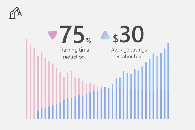
The benefits of adopting mixed reality today are significant. Based on the Microsoft-commissioned Forrester Total Economic Impact (TEI) report (“HoloLens 2 TEI study”), HoloLens 2 is delivering 177 percent return on investment (ROI) and a net present value (NPV) of $7.6 million over three years with a payback of 13 months. According to the HoloLens 2 TEI study, manufacturing organizations that have deployed mixed reality solutions on HoloLens 2 have:
Reduced training time by 75 percent, at an average savings of $30 per labor hour.
Saved an average of $3,500 per avoided expert trip.
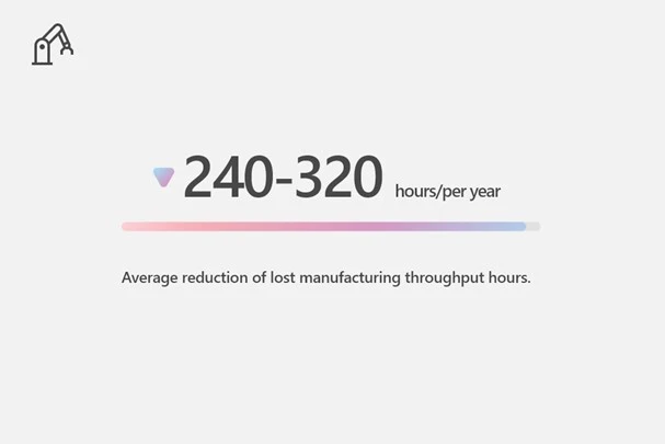
Avoided 240 to 320 hours of average lost throughput per year.
Increase productivity with remote inspection and audits
Dynamics 365 mixed reality is reducing the requirement to fly in an expert technician and/or an auditor on site to conduct an inspection. With Dynamics 365 Remote Assist on HoloLens 2, manufacturing companies can conduct routine inspections and audits with remote experts from any place in the world at any time. Manufacturers can deliver real-time, interactive guidance from experts located anywhere in the world right to their employees on the factory floor. This solution allows onsite workers to collaborate with remote leaders and experts to solve business problems in real-time, using 3D annotations to access, share, and bring critical information into view. With accurate real-world overlay of 3D assets, instructions, and collaborative markup, workers are free to see their surroundings and use both hands during inspections.
Dynamics 365 Remote Assist on HoloLens 2 enables manufacturer organizations to conduct site visits, inspections, maintenance, and repairs remotelyboosting efficiency and reducing costs. According to the HoloLens 2 TEI study, manufacturers saved an average of $3,500 per avoided expert trip.
Eaton, a multinational power management company, sought a solution to enable the company to conduct audits remotely. Traditionally, auditors had to travel to plants to conduct audits but during the COVID-19 pandemic travel was brought to a standstill and travel was restricted. With Dynamics 365 Remote Assist on HoloLens 2, employees can walk through the audit checklist with the remote auditor and ensure that employees are following safety guidelines. Since launching Dynamics 365 Remote Assist on HoloLens 2, Eaton is averaging more than 50 remote sessions per month across all global sites saving hundreds of thousands of dollars on travel-related expenses and empowering Eaton to pay-off its mixed-reality investment within five months.
“Using Remote Assist on HoloLens, we’re bringing the outside viewer perspective into the plant. Let’s say they are checking a quality dimension. If someone on the call has been on another Gemba walk in another site, they can say, ‘You should contact plant XYZ, because they do a similar measurement, but they’re using an automated process.”Alexandre Georgetti, Director of Eaton’s Vehicle Group Manufacturing Strategy. Read more about Eaton’s story here.
Address manufacturing skills gap with guided assembly and training
Dynamics 365 mixed reality is reducing the knowledge gap and helping enterprises adapt at the speed of change. Using Dynamics 365 Guides on HoloLens 2, manufacturing companies are accelerating learning, standardizing processes, and reducing errors with step-by-step instructions. Simply use your PC and the Microsoft HoloLens app to author instructions and easily place 2D and 3D content in the real-world environment, showing users how and where to complete tasks.
Dynamics 365 Guides on HoloLens 2 empowers manufacturing organizations to offer expansive training programs that teach skills and processes that are specific to their offerings and production needs. Furthermore, manufacturers see direct improvements in learning and retention, quality of work and downtime, and training costs savings. According to the HoloLens 2 TEI study, manufacturers reduced training time by 75 percent, at an average savings of $30 per labor hour.
Toyota, a multinational automobile manufacturer, produces over a million vehicles each year in North America and depends on solid training programs that ensure team members are building every car to precise specifications. Traditionally, trainers worked one-on-one with team members, demonstrating a process, and then watching them replicate it. Toyota found this approach to be inefficient and susceptible to bottlenecks. With Dynamics 365 Guides on HoloLens 2, trainers create training materials and allow team members to train independently and understand the steps involved and repeating any necessary motions numerous times to develop muscle memory while allowing for one trainer supervisor to supervise multiple trainees at the same time. Since deploying Dynamics 365 mixed reality solutions on HoloLens 2, Toyota has reduced inspection time by 20 percent.
“Our training efficiency is increased, trainers and trainees are receptive to the technology, and they rank Dynamics 365 Guides on HoloLens 2 as their preferred way to learn.”Zach Reeder, Technology Development Engineer at Toyota Motor North America. Read more about Toyota’s story here.
Connect workers with experts to enable always on service
Dynamics 365 mixed reality is helping enterprises deliver exceptional service with personalized customer experiences. Dynamics 365 Remote Assist on HoloLens 2 connects field technicians with remote experts for a seamless collaboration that includes content capture abilities, interactive annotations, and contextual data overlays for easier repairs and fixes. Equip field technicians with all the important, relevant information directly into their line of sight, creating actionable experiences for employees.
Dynamics 365 Remote Assist on HoloLens 2 improves field task efficiency, reduces rework, and improves first-time fix ratesincreasing capacity for work and improving customer outcomes. According to the HoloLens 2 TEI study, manufacturers avoided 240 to 320 hours of average lost throughput per year.
L’Oral, one of the top multination cosmetics manufacturers with employees in 150 countries, has a wide range of products that require sophisticated machinery for production and packaging. When a machine requires service, L’Oreal flies out an expert to address the issue, increasing downtime machine and travel costs. To solve this challenge, L’Oreal deployed Dynamics 365 Remote Assist on HoloLens 2 to enable remote experts to effectively collaborate with frontline workers to resolve the issue expeditiously and reduce operational costs. With Dynamics 365 Remote Assist on HoloLens 2, remote experts can see what the technician sees and react to the same image with annotations and share critical information in real-time. Since deploying Dynamics 365 Remote Assist on HoloLens 2, L’Oreal has reduced downtime by 50 percent.
“The time we spend on diagnostics and resolving issues has been cut in half. This has led directly to lower operational costs. It has also allowed us to be more agile and flexible”Georges-Alban Farges, Industrial Performance Manager at L’Oral. Read about L’Oral’s story here.
Next steps
Stay tuned as we continue this blog series with a deep dive spotlight on healthcare, education, architecture, engineering, and construction industries. In the meantime, learn more about mixed reality applications on HoloLens 2 and get started today:
Request a Dynamics 365 Mixed Reality demo on Microsoft HoloLens 2. Book an appointment with our Microsoft Stores team today. Select ‘Other’ under Choose topic and reference HoloLens 2 demo in “What can we help with”.
This article is contributed. See the original author and article here.
As the shift to hybrid work becomes a reality, it is clear that the workplace today is different than it was two years ago. Employees’ expectations continue to evolve as they reconsider their “worth it” equation.
The threat actor harvested credentials of third-party commercial organizations by sending spearphishing emails that contained a PDF attachment. The PDF attachment contained a shortened URL that, when clicked, led users to a website that prompted the user for their email address and password. The threat actor harvested credentials of Energy Sector targets by sending spearphishing emails with a malicious Microsoft Word document or links to the watering holes created on compromised third-party websites.
Note: this activity also applies to:
Tactic: Reconnaissance [TA0043], Technique: Phishing for Information [T1598]:
Software Configuration: implement configuration changes to software (other than the operating system) to mitigate security risks associated to how the software operates.
User Training: train users to be aware of access or manipulation attempts by an adversary to reduce the risk of successful spearphishing, social engineering, and other techniques that involve user interaction.
The threat actor created watering holes on compromised third-party organizations’ domains.
This activity typically takes place outside the visibility of target organizations, making detection of this behavior difficult. Ensure that users browse the internet securely. Prevent intentional and unintentional download of malware or rootkits, and users from accessing infected or malicious websites. Treat all traffic as untrusted, even if it comes from a partner website or popular domain.
The threat actor obtained access to Energy Sector targets by leveraging compromised third-party infrastructure and previously compromised Energy Sector credentials against remote access services and infrastructure—specifically VPN, RDP, and Outlook Web Access—where MFA was not enabled.
Network Segmentation: architect sections of the network to isolate critical systems, functions, or resources. Use physical and logical segmentation to prevent access to potentially sensitive systems and information. Use a DMZ to contain any internet-facing services that should not be exposed from the internal network.
MFA: enforce use of two or more pieces of evidence (such as username and password plus a token, e.g., a physical smart card or token generator) to authenticate to a system.
Privileged Account Management: manage the creation of, modification of, use of, and permissions associated with privileged accounts, including SYSTEM and root.
Update Software: perform regular software updates to mitigate exploitation risk.
Exploit Protection: use capabilities to detect and block conditions that may lead to or be indicative of a software exploit occurring.
Application Isolation and Sandboxing: restrict execution of code to a virtual environment on or in transit to an endpoint system.
The threat actor installed VPN clients on compromised third-party targets to connect to Energy Sector networks.
Network Segmentation: architect sections of the network to isolate critical systems, functions, or resources. Use physical and logical segmentation to prevent access to potentially sensitive systems and information. Use a DMZ to contain any internet-facing services that should not be exposed from the internal network.
MFA: enforce use of two or more pieces of evidence (such as username and password plus a token, e.g., a physical smart card or token generator) to authenticate to a system.
Limit Access to Resource Over Network: prevent access to file shares, remote access to systems, and unnecessary services. Mechanisms to limit access may include use of network concentrators, RDP gateways, etc.
Disable or Remove Program: remove or deny access to unnecessary and potentially vulnerable software to prevent abuse by adversaries.
Command and Scripting Interpreter: PowerShell [T1059.001]
During an RDP session, the threat actor used a PowerShell Script to create an account within a victim’s Microsoft Exchange Server.
Note: this activity also applies to:
Tactic: Persistence [TA0003], Technique: Create Account: Local Account [T1136.001]
Antivirus/Antimalware: use signatures or heuristics to detect malicious software.
Code Signing: enforce binary and application integrity with digital signature verification to prevent untrusted code from executing.
Disable or Remove Program: remove or deny access to unnecessary and potentially vulnerable software to prevent abuse by adversaries.
Privileged Account Management: manage the creation of, modification of, use of, and permissions associated with privileged accounts, including SYSTEM and root.
Command and Scripting Interpreter: Windows Command Shell [T1059.003]
The threat actor used a JavaScript with an embedded Command Shell script to:
Create a local administrator account;
Disable the host-based firewall;
Globally open port 3389 for RDP access; and
Attempt to add the newly created account to the administrators group to gain elevated privileges.
The threat actor created a Scheduled Task to automatically log out of a newly created account every eight hours.
Audit: audit or scan systems, permissions, insecure software, insecure configurations, etc., to identify potential weaknesses.
Harden Operating System Configuration: make configuration changes related to the operating system or a common feature of the operating system that result in system hardening against techniques.
Privileged Account Management: manage the creation of, modification of, use of, and permissions associated with privileged accounts, including SYSTEM and root.
User Account Management: manage the creation of, modification of, use of, and permissions associated with user accounts.
The threat actor created local administrator accounts on previously compromised third-party organizations for reconnaissance and to remotely access Energy Sector targets. MFA: enforce use of two or more pieces of evidence (such as username and password plus a token, e.g., a physical smart card or token generator) to authenticate to a system.
MFA: enforce use of two or more pieces of evidence (such as username and password plus a token, e.g., a physical smart card or token generator) to authenticate to a system.
Privileged Account Management: manage the creation of, modification of, use of, and permissions associated with privileged accounts, including SYSTEM and root.
The threat actor created webshells on Energy Sector targets’ publicly accessible email and web servers.
Detect: the portion of the webshell that is on the server may be small and look innocuous. Process monitoring may be used to detect Web servers that perform suspicious actions such as running cmd.exe or accessing files that are not in the Web directory. File monitoring may be used to detect changes to files in the Web directory of a Web server that do not match with updates to the Web server’s content and may indicate implantation of a Web shell script. Log authentication attempts to the server and any unusual traffic patterns to or from the server and internal network.
Indicator Removal on Host: Clear Windows Event Logs [T1070.001]
The threat actor created new accounts on victim networks to perform cleanup operations. The accounts created were used to clear the following Windows event logs: System, Security, Terminal Services, Remote Services, and Audit.
The threat actor also removed applications they installed while they were in the network along with any logs produced. For example, the VPN client installed at one third-party commercial facility was deleted along with the logs that were produced from its use. Finally, data generated by other accounts used on the systems accessed were deleted.
Note: this activity also applies to:
Tactic: Persistence [TA0003], Technique: Create Account: Local Account [T1136.001]
Encrypt Sensitive Information: protect sensitive information with strong encryption.
Remote Data Storage: use remote security log and sensitive file storage where access can be controlled better to prevent exposure of intrusion detection log data or sensitive information.
Restrict File and Directory Permissions: restrict access by setting directory and file permissions that are not specific to users or privileged accounts.
Indicator Removal on Host: File Deletion [T1070.004]
The threat actor cleaned up target networks by deleting created screenshots and specific registry keys.
The threat actor also deleted all batch scripts, output text documents, and any tools they brought into the environment, such as scr.exe.
Monitor: monitoring for command-line deletion functions to correlate with binaries or other files that an adversary may drop and remove may lead to detection of malicious activity. Another good practice is monitoring for known deletion and secure deletion tools that are not already on systems within an enterprise network that an adversary could introduce. Some monitoring tools may collect command-line arguments, but may not capture DEL commands since DEL is a native function within cmd.exe.
After downloading tools from a remote server, the threat actor renamed the extensions.
Restrict File and Directory Permissions: restrict access by setting directory and file permissions that are not specific to users or privileged accounts.
Code Signing: enforce binary and application integrity with digital signature verification to prevent untrusted code from executing.
Execution Prevention: block execution of code on a system through application control, and/or script blocking.
The threat actor used password-cracking techniques to obtain the plaintext passwords from obtained credential hashes.
The threat actor dropped and executed open-source and free password cracking tools such as Hydra, SecretsDump, and CrackMapExec, and Python.
MFA: enforce use of two or more pieces of evidence (such as username and password plus a token, e.g., a physical smart card or token generator) to authenticate to a system.
Password Policies: set and enforce secure password policies for accounts.
Microsoft Word attachments sent via spearphishing emails leveraged legitimate Microsoft Office functions for retrieving a document from a remote server over Server Message Block (SMB) using Transmission Control Protocol ports 445 or 139. As a part of the standard processes executed by Microsoft Word, this request authenticates the client with the server, sending the user’s credential hash to the remote server before retrieving the requested file. (Note: transfer of credentials can occur even if the file is not retrieved.)
Password Policies: set and enforce secure password policies for accounts.
Filter Network Traffic: use network appliances to filter ingress or egress traffic and perform protocol-based filtering. Configure software on endpoints to filter network traffic.
The threat actor’s watering hole sites contained altered JavaScript and PHP files that requested a file icon using SMB from an IP address controlled by the threat actors.
The threat actor manipulated LNK files to repeatedly gather user credentials. Default Windows functionality enables icons to be loaded from a local or remote Windows repository. The threat actor exploited this built-in Windows functionality by setting the icon path to a remote server controller by the actors. When the user browses to the directory, Windows attempts to load the icon and initiate an SMB authentication session. During this process, the active user’s credentials are passed through the attempted SMB connection.
OS Credential Dumping: Local Security Authority Subsystem Service (LSASS) Memory [T1003.001]
The threat actor used an Administrator PowerShell prompt to enable the WDigest authentication protocol to store plaintext passwords in the LSASS memory. With this enabled, credential harvesting tools can dump passwords from this process’s memory.
Operating System Configuration: make configuration changes related to the operating system or a common feature of the operating system that result in system hardening against techniques.
Password Policies: set and enforce secure password policies for accounts.
Privileged Account Management: manage the creation of, modification of, use of, and permissions associated with privileged accounts, including SYSTEM and root.
Privileged Process Integrity: protect processes with high privileges that can be used to interact with critical system components through use of protected process light, anti-process injection defenses, or other process integrity enforcement measures.
User Training: train users to be aware of access or manipulation attempts by an adversary to reduce the risk of successful spearphishing, social engineering, and other techniques that involve user interaction.
Credential Access Protection: use capabilities to prevent successful credential access by adversaries; including blocking forms of credential dumping.
The threat actor collected the files ntds.dit. The file ntds.dit is the Active Directory (AD) database that contains all information related to the AD, including encrypted user passwords.
Monitor: monitor processes and command-line arguments for program execution that may be indicative of credential dumping, especially attempts to access or copy the NTDS.dit.
Privileged Account Management: manage the creation of, modification of, se of, and permissions associated with privileged accounts, including SYSTEM and root.
User Training: train users to be aware of access or manipulation attempts by an adversary to reduce the risk of successful spearphishing, social engineering, and other techniques that involve user interaction.
The threat actor used privileged credentials to access the Energy Sector victim’s domain controller. Once on the domain controller, the threat actors used batch scripts dc.bat and dit.bat to enumerate hosts, users, and additional information about the environment.
Tactic: Discovery [TA0007], Technique: System Owner/User Discovery [T1033]
Monitor: normal, benign system and network events related to legitimate remote system discovery may be uncommon, depending on the environment and how they are used.
Monitor processes and command-line arguments for actions that could be taken to gather system and network information.
Monitor for processes that can be used to discover remote systems, such as ping.exe and tracert.exe, especially when executed in quick succession.
The threat actor accessed workstations and servers on corporate networks that contained data output from control systems within energy generation facilities. The threat actors accessed files pertaining to ICS or supervisory control and data acquisition (SCADA) systems.
The actor targeted and copied profile and configuration information for accessing ICS systems on the network. The threat actor copied Virtual Network Connection (VNC) profiles that contained configuration information on accessing ICS systems and took screenshots of a Human Machine Interface (HMI).
Note: this activity also applies to
Tactic: Discovery [TA0007], Technique File and Directory Discovery [T1083]
The actor used dirsb.bat to gather folder and file names from hosts on the network.
Note: this activity also applies to:
Tactic: Execution [TA0002], Command and Scripting Interpreter: Windows Command Shell [T1059.003]
This type of attack technique cannot be easily mitigated with preventive controls since it is based on the abuse of system features. Monitor processes and command-line arguments for actions that could be taken to gather system and network information. Remote access tools with built-in features may interact directly with the Windows API to gather information.
The threat actor conducted reconnaissance operations within the network. The threat actor focused on identifying and browsing file servers within the intended victim’s network.
Network Intrusion Prevention: use intrusion detection signatures to block traffic at network boundaries.
Network Segmentation: architect sections of the network to isolate critical systems, functions, or resources. Use physical and logical segmentation to prevent access to potentially sensitive systems and information. Use a DMZ to contain any internet-facing services that should not be exposed from the internal network.
Operating System Configuration: make configuration changes related to the operating system or a common feature of the operating system that result in system hardening against techniques.
Privileged Account Management: manage the creation of, modification of, use of, and permissions associated with privileged accounts, including SYSTEM and root.
User Account Management: manage the creation of, modification o, se of, and permissions associated with user accounts.
Disable or Remove Feature or Program: remove or deny access to unnecessary and potentially vulnerable software to prevent abuse by adversaries.
Audit: audit or scan systems, permissions, insecure software, insecure configurations, etc. to identify potential weaknesses.
MFA: enforce use of two or more pieces of evidence (such as username and password plus a token, e.g., a physical smart card or token generator) to authenticate to a system.
Limit Access to Resource Over Network: prevent access to file shares, remote access to systems, and unnecessary services. Mechanisms to limit access may include use of network concentrators, RDP gateways, etc.
Filter Network Traffic: use network appliances to filter ingress or egress traffic and perform protocol-based filtering. Configure software on endpoints to filter network traffic.
Limit Software Installation: block users or groups from installing unapproved software.
The threat actor collected the Windows SYSTEM registry hive file, which contains host configuration information.
Monitor: monitor processes and command-line arguments for actions that could be taken to collect files from a system. Remote access tools with built-in features may interact directly with the Windows API to gather data.
Data may also be acquired through Windows system management tools such as WMI and PowerShell.
Archive Collected Data: Archive via Utility [T1560.001]
The threat actor compressed the ntds.dit file and the SYSTEM registry hive they had collected into archives named SYSTEM.zip and comps.zip.
Audit: audit or scan systems, permissions, insecure software, insecure configurations, etc. to identify potential weaknesses.
The threat actor used Windows’ Scheduled Tasks and batch scripts, to execute scr.exe and collect additional information from hosts on the network. The tool scr.exe is a screenshot utility that the threat actor used to capture the screen of systems across the network.
Network Segmentation: architect sections of the network to isolate critical systems, functions, or resources. Use physical and logical segmentation to prevent access to potentially sensitive systems and information. Use a DMZ to contain any internet-facing services that should not be exposed from the internal network.
MFA: enforce use of two or more pieces of evidence (such as username and password plus a token, e.g., a physical smart card or token generator) to authenticate to a system.
Limit Access to Resource Over Network: prevent access to file shares, remote access to systems, and unnecessary services. Mechanisms to limit access may include use of network concentrators, RDP gateways, etc.
Disable or Remove Feature or Program: remove or deny access to unnecessary and potentially vulnerable software to prevent abuse by adversaries.
The actor used batch scripts labeled pss.bat and psc.bat to run the PsExec tool. PsExec was used to execute scr.exe across the network and to collect screenshots of systems in a text file.
The threat actor downloaded tools from a remote server.
Monitor: monitor for file creation and files transferred into the network. Unusual processes with external network connections creating files on-system may be suspicious. Use of utilities, such as File Transfer Protocol, that does not normally occur may also be suspicious.
Analyze network data for uncommon data flows (e.g., a client sending significantly more data than it receives from a server). Processes utilizing the network that do not normally have network communication or have never been seen before are suspicious.
Analyze packet contents to detect communications that do not follow the expected protocol behavior for the port that is being used.
Use intrusion detection signatures to block traffic at network boundaries.
This article is contributed. See the original author and article here.
CISA, the Federal Bureau of Investigation, and the Department of Energy have released a joint Cybersecurity Advisory (CSA) detailing campaigns conducted by state-sponsored Russian cyber actors from 2011 to 2018 that targeted U.S. and international Energy Sector organizations. The CSA highlights historical tactics, techniques, and procedures as well as mitigations Energy Sector organizations can take now to protect their networks.


Recent Comments