A Future With Safer Roads: Automatic Wheel Lug Nut Detection Using Machine Learning at the Edge

by Contributed | Jul 17, 2021 | Technology

This article is contributed. See the original author and article here.

By Evan Rust and Zin Thein Kyaw

Introduction

Wheel lug nuts are such a tiny part of the overall automobile assembly that they’re easy to overlook, but yet serve a critical function in the safe operation of an automobile. In fact, it is not safe to drive even with one lug nut missing. A single missing lug nut will cause increased pressure on the wheel, in turn causing damage to the wheel bearings, studs, and make the other lug nuts fall off. 

Over the years there have been a number of documented safety recalls and issues around wheel lug nuts. In some cases, it was only identified after the fact that the automobile manufacturer had installed incompatible lug nut types with the wheel or had been inconsistent in installing the right type of lug nut. Even after delivery, after years of wear and tear, the lug nuts may become loose and may even fall off which would cause instability for an automobile to be in service. To reduce these incidents of quality control at manufacturing and maintenance in the field, there is a huge opportunity to leverage machine learning at the edge to automate wheel lug nut detection. 

This motivated us to create a proof-of-concept reference project for automating wheel lug nut detection by easily putting together a USB webcam, Raspberry Pi 4, Microsoft Azure IoT, and Edge Impulse, creating an end-to-end wheel lug nut detection system using Object Detection. This example use case and other derivatives will find a home in many industrial IoT scenarios where embedded Machine Learning can help improve the efficiency of factory automation and quality control processes including predictive maintenance. 

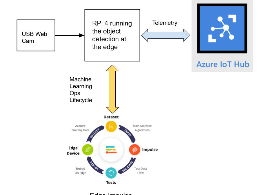
This reference project will serve as a guide for quickly getting started with Edge Impulse on the Raspberry Pi 4 and Azure IoT, to train a model that detects lug nuts on a wheel and sends inference conclusions to Azure IoT as shown in the block diagram below:

Design Concept: Edge Impulse and Azure IoT

Edge Impulse is an embedded machine learning platform that allows you to manage the entire Machine Learning Ops (MLOps) lifecycle which includes 1) Data Acquisition, 2) Signal Processing, 3) ML Training, 4) Model Testing, and 5) Creating a deployable model that can run efficiently on an edge device. 

For the edge device, we chose to use the Raspberry Pi 4 due to its ubiquity and available processing power for efficiently running more sophisticated machine learning models such as object detection. By running the object detection model on the Raspberry Pi 4, we can optimize the network bandwidth connection to Azure IoT for robustness and scalability by only sending the inference conclusions, i.e. “How many lug nuts are on the wheel?”. Once the inference conclusions are available at the Azure IoT level, it becomes straightforward to feed these results into your business applications that can leverage other Azure services such as Azure Stream Analytics and Power BI.

In the next sections we’ll discuss how you can set this up yourself with the following items:

• Raspberry Pi 4


• USB webcam (such as a Logitech HD webcam)


• Edge Impulse account 


• Azure IoT Hub instance
  
  

Setting Up the Hardware

We begin by setting up the Raspberry Pi 4 to connect to a Wi-Fi network for our network connection, configuring it for camera support, and installing the Edge Impulse Linux CLI (command line interface) tools on the Raspberry Pi 4. This will allow the Raspberry Pi 4 to directly connect to Edge Impulse for data acquisition and finally, deployment of the wheel lug nut detection model. 

For starters, you’ll need a Raspberry Pi 4 with an up-to-date Raspberry Pi OS image that can be found here. After flashing this image to an SD card and adding a file named ‘wpa_supplicant.conf’:

ctrl_interface=DIR=/var/run/wpa_supplicant GROUP=netdev
update_config=1
country=<Insert 2 letter ISO 3166-1 country code here>
network={
 ssid="<Name of your wireless LAN>"
 psk="<Password for your wireless LAN>"
}

along with an empty file named ‘ssh’ (both within the ‘/boot’ directory), you can go ahead and power up the board. 

Once you’ve successfully SSH’d into the device with

ssh pi@<IP_ADDRESS>

and the password ‘raspberry’, it’s time to install the dependencies for the Edge Impulse Linux SDK. Simply run the next three commands to set up the NodeJS environment and everything else that’s required for the edge-impulse-linux wizard: 

curl -sL https://deb.nodesource.com/setup_12.x | sudo bash -
sudo apt install -y gcc g++ make build-essential nodejs sox gstreamer1.0-tools gstreamer1.0-plugins-good gstreamer1.0-plugins-base gstreamer1.0-plugins-base-apps
npm config set user root && sudo npm install edge-impulse-linux -g --unsafe-perm

For more details on setting up the Raspberry Pi 4 with Edge Impulse, visit this link.

Since this project deals with images, we’ll need some way to capture them. The wizard supports both the Pi camera modules and standard USB webcams, so make sure to enable the camera module first with

sudo raspi-config

if you plan on using one. With that completed, go to Edge Impulse and create a new project, then run the wizard with 

edge-impulse-linux

and make sure your device appears within the Edge Impulse Studio’s device section after logging in and selecting your project.

Data Acquisition

Training accurate production ready machine learning models requires feeding plenty of varied data, which means a lot of images are typically required. For this proof-of-concept, we captured around 145 images of a wheel that had lug nuts on it. The Edge Impulse Linux daemon allows you to directly connect the Raspberry Pi 4 to Edge Impulse and take snapshots using the USB webcam. 

Using the Labeling queue in the Data Acquisition page we then easily drew bounding boxes around each lug nut within every image, along with every wheel. To add some test data we went back to the main Dashboard page and clicked the ‘Rebalance dataset’ button that moves 20% of the training data to the test data bin. 

Impulse Design and Model Training

Now that we have plenty of training data, it’s time to design and build our model. The first block in the Impulse Design is an Image Data block, and it scales each image to a size of ‘320’ by ‘320’ pixels. 

Next, image data is fed to the Image processing block that takes the raw RGB data and derives features from it.

Finally, these features are used as inputs to the MobileNetV2 SSD FPN-Lite Transfer Learning Object Detection model that learns to recognize the lug nuts. The model is set to train for ’25’ cycles at a learning rate of ‘.15’, but this can be adjusted to fine-tune for accuracy. As you can see from the screenshot below, the trained model indicates a precision score of 97.9%.

Model Testing

If you’ll recall from an earlier step we rebalanced the dataset to put 20% of the images we collected to be used for gauging how our trained model could perform in the real world. We use the model testing page to run a batch classification and see how we expect our model to perform. The ‘Live Classification’ tab will also allow you to acquire new data direct from the Raspberry Pi 4 and see how the model measures up against the immediate image sample. 

Versioning

An MLOps platform would not be complete without a way to archive your work as you iterate on your project. The ‘Versioning’ tab allows you to save your entire project including the entire dataset so you can always go back to a “known good version” as you experiment with different neural network parameters and project configurations. It’s also a great way to share your efforts as you can designate any version as ‘public’ and other Edge Impulse users can clone your entire project and use it as a springboard to add their own enhancements. 

Deploying Models

In order to verify that the model works correctly in the real world, we’ll need to deploy it to the Raspberry Pi 4. This is a simple task thanks to the Edge Impulse CLI, as all we have to do is run

edge-impulse-linux-runner 

which downloads the model and creates a local webserver. From here, we can open a browser tab and visit the address listed after we run the command to see a live camera feed and any objects that are currently detected. Here’s a sample of what the user will see in their browser tab:

Sending Inference Results to Azure IoT Hub

With the model working locally on the Raspberry Pi 4, let’s see how we can send the inference results from the Raspberry Pi 4 to an Azure IoT Hub instance. As previously mentioned, these results will enable business applications to leverage other Azure services such as Azure Stream Analytics and Power BI. On your development machine, make sure you’ve installed the Azure CLI and have signed in using ‘az login’. Then get the name of the resource group you’ll be using for the project. If you don’t have one, you can follow this guide on how to create a new resource group.

After that, return to the terminal and run the following commands to create a new IoT Hub and register a new device ID:

az iot hub create --resource-group <your resource group> --name <your IoT Hub name>
az extension add --name azure-iot
az iot hub device-identity create --hub-name <your IoT Hub name> --device-id <your device id>

Retrieve the connection string the Raspberry Pi 4 will use to connect to Azure IoT with: 

az iot hub device-identity connection-string show --device-id <your device id> --hub-name <your IoT Hub name>

Now it’s time to SSH into the Raspberry Pi 4 and set the connection string as an environment variable with:

export IOTHUB_DEVICE_CONNECTION_STRING="<your connection string here>"

Then, add the necessary Azure IoT device libraries with:

pip install azure-iot-device

(Note: if you do not set the environment variable or pass it in as an argument the program will not work!) The connection string contains the information required for the Raspberry Pi 4 to establish a connection with the Azure IoT Hub service and communicate with it. You can then monitor output in the Azure IoT Hub with:

az iot hub monitor-events --hub-name <your IoT Hub name> --output table

or in the Azure Portal.

To make sure it works, download and run this example on the Raspberry Pi 4 to make sure you can see the test message.

For the second half of deployment, we’ll need a way to customize how our model is used within the code. Edge Impulse provides a Python SDK for this purpose. On the Raspberry Pi 4 install it with 

sudo apt-get install libatlas-base-dev libportaudio0 libportaudio2 libportaudiocpp0 portaudio19-dev
pip3 install edge_impulse_linux -i https://pypi.python.org/simple

We’ve made available a simple example on the Raspberry Pi 4 that sets up a connection to the Azure IoT Hub, runs the model, and sends the inference results to Azure IoT.

Once you’ve either downloaded the zip file or cloned the repo into a folder, get the model file by running 

edge-impulse-linux-runner --download modelfile.eim

inside of the folder you just created from the cloning process. This will download a file called ‘modelfile.eim’. Now, run the Python program with 

python lug_nut_counter.py ./modelfile.eim -c <LUG_NUT_COUNT>

where <LUG_NUT_COUNT> is the correct number of lug nuts that should be attached to the wheel (you might have to use ‘python3’ if both Python 2 and 3 are installed).

Now whenever a wheel is detected the number of lug nuts is calculated. If this number falls short of the target, a message is sent to the Azure IoT Hub.

And by only sending messages when there’s something wrong, we can prevent an excess amount of bandwidth from being taken due to empty payloads.

Conclusion

We’ve just scratched the surface with wheel lug nut detection. Imagine utilizing object detection for other industrial applications in quality control, detecting ripe fruit amongst rows of crops, or identifying when machinery has malfunctioned with devices powered by machine learning.

With any hardware, Edge Impulse, and Microsoft Azure IoT, you can design comprehensive embedded machine learning models, deploy them on any device, while authenticating each and every device with built-in security. You can set up individual identities and credentials for each of your connected devices to help retain the confidentiality of both cloud-to-device and device-to-cloud messages, revoke access rights for specific devices, upgrade device firmware remotely, and benefit from advanced analytics on devices running offline or with intermittent connectivity.

The complete Edge Impulse project is available here for you to see how easy it is to start building your own embedded machine learning projects today using object detection. We look forward to your feedback at hello@edgeimpulse.com or on our forum.

Design a Azure IoT Indoor Air Quality monitoring platform from scratch

by Contributed | Jul 17, 2021 | Technology

This article is contributed. See the original author and article here.

This article is the first part of a series which explores an end-to-end pipeline to deploy an Air Quality Monitoring application using off-the-market sensors, Azure IoT Ecosystem and Python. We will begin by looking into what is the problem, some terminology, prerequisites, reference architecture, and an implementation. 

Indoor Air Quality – why does it matter and how to measure it with IoT?

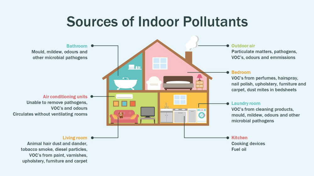
Most people think of air pollution as an outdoor problem, but indoor air quality has a major impact on health and well-being since the average American spends about 90 percent of their time indoors. Proper ventilation is one of the most important considerations for maintaining good indoor air quality. Poor indoor air quality is known to be harmful to vulnerable groups such as the elderly, children or those suffering chronic respiratory and/or cardiovascular diseases. Here is a quick visual on some sources of indoor air pollution.

Post Covid-19, we are in a world where awareness of our indoor environments is key for survival. Here in Canada we are quite aware of the situation, which is why we have a set of guidlines from the Government of Canada, and a recent white paper from Public Health Ontario. The American Medical Association has put up this excellent document for reference. So now that we know what the problem is, how do we go about solving it? To solve something we must be able to measure it and currently we have some popular metrics to measure air quality, viz. IAQ and VOC.

So what are IAQ and VOC exactly?

Indoor air quality (IAQ) is the air quality within and around buildings and structures. IAQ is known to affect the health, comfort, and well-being of building occupants. IAQ can be affected by gases (including carbon monoxide, radon, volatile organic compounds), particulates, microbial contaminants (mold, bacteria), or any mass or energy stressor that can induce adverse health conditions. IAQ is part of indoor environmental quality (IEQ), which includes IAQ as well as other physical and psychological aspects of life indoors (e.g., lighting, visual quality, acoustics, and thermal comfort). In the last few years IAQ has received increasing attention from environmental governance authorities and IAQ-related standards are getting stricter. Here is a IAQ blog infographic if you’d like to read.

Volatile organic compounds (VOC) are organic chemicals that have a high vapour pressure at room temperature. High vapor pressure correlates with a low boiling point, which relates to the number of the sample’s molecules in the surrounding air, a trait known as volatility. VOC’s are responsible for the odor of scents and perfumes as well as pollutants. VOCs play an important role in communication between animals and plants, e.g. attractants for pollinators, protection from predation, and even inter-plant interactions. Some VOCs are dangerous to human health or cause harm to the environment. Anthropogenic VOCs are regulated by law, especially indoors, where concentrations are the highest. Most VOCs are not acutely toxic, but may have long-term chronic health effects. Refer to this and this for vivid details.

The point is, in a post pandemic world, having a centralized air quality monitoring system is an absolute necessity. The need for collecting this data and using the insights from it is crucial to living better. And this is where Azure IoT comes in. In this series we are going to explore how to create the moving parts of this platform with ‘minimum effort‘. In this first part, we are goiing to concentrate our efforts on the overall architecture, hardware/software requirements, and IoT edge module creation. 

Prerequisites

To accomplish our goal we will ideally need to meet a few basic criteria. Here is a short list.

1. Air Quality Sensor (link)


2. IoT Edge device (link)


3. Active Azure subscription (link)


4. Development machine


5. Working knowledge of Python, Sql, Docker, Json, IoT Edge runtime, VSCode


6. Perseverance

Lets go into a bit of details about the aforementioned points since there are many possibilities. 

Air Quality Sensor

This is the sensor that emits the actual IAQ/VOC+ data. Now, there are a lot of options in this category, and technically they should be producing the same results. However, the best sensors in the market are Micro-Electro-Mechanical Systems (MEMS). MEMS technology uses semiconductor fabrication processes to produce miniaturized mechanical and electro-mechanical elements that range in size from less than one micrometer to several millimeters. MEMS devices can vary from relatively simple structures with no moving elements, to complex electromechanical systems with multiple moving elements. My choice was uThing::VOC™ Air-Quality USB sensor dongle. This is mainly to ensure high quality output and ease of interfacing, which is USB out of the box, and does not require any installation. Have a look at the list of features available on this dongle. The main component is a Bosch proprietary algorithm and the BME680 sensor that does all the hard work. Its basically plug-and-play.  The data is emitted in Json format and is available at an interval of 3 milliseconds on the serial port of your device. In my case it was /dev/ttyACM0, but could be different in yours.

IoT Edge device

This is the edge system. where the sensor is plugged in. Typical choices are windows or linux. If you are doing windows, be aware some of these steps may be different and you have to figure those out. However, in my case I am using ubuntu 20.04 installed on an Intel NUC. The reason I chose the NUC is because many IoT modules require an x86_64 machine, which is not available in ARM devices (Jetson, Rasp Pi, etc.) Technically this should work on ANY edge device with a usb port, but for example windows has an issue mounting serial ports onto containers. I suggest better stick with linux unless its a client requirement.

Active Azure subscription

Surely, you will need this one, but as we know Azure has this immense suit of products, and while ideally we want to have everything, it may not be practically feasible. For practical purposes you might have to ask for access to particular services, meaning you have to know ahead exactly which ones you want to use. Of course the list of required services will vary between use cases, so we will begin with just the bare minimum. We will need the following:

• Azure IoT Hub (link)


• Azure Container Registry (link)


• Azure blob storage (link)


• Azure Streaming Analytics (link)(future article)


• Power BI / React App (link)(future article)


• Azure Linux VM (link)(optional)

A few points before we move to the next prerequisite. For IoT hub you can use free tier for experiments, but I will recommend to use the standard tier instead. For ACR get the usual tier and generate username password. For storageaccount its the standard tier. The ASA and BI products will be used in the reference architecture, but is not discussed in this article. The final service Azure VM is an interesting one. Potentially all the codebase can be run using VM, but this is only good for simulations. However, note that it is an equally good idea to experiment with VMs first as they have great integration and ease the learning curve.

Development machine

The development machine can be literally anything from which you have ssh access to the edge device. From an OS perspective it can be windows, linux, raspbian, mac etc. Just remember two things – use a good IDE (a.k.a VSCode) and make sure docker can be run on it, optionally with priviliges. In my case I am using a Startech KVM, so I can shift between my windows machine and the actual edge device for development purposes, but it is not neccessary.

Working knowledge of Python, Sql, Docker, Json, IoT Edge runtime, VSCode

This is where it gets tricky. Having a mix of these knowledge is somewhat essential to creating and scaling this platform. However, I understand you may not be having proficiency in all of these. On that note, I can tell from experience that being from a data engineering background has been extremely beneficial for me. In any case, you will need some python skills, some sql, and Json. Even knowing how to use the VSCode IoT extension is non-trivial. One notable mention is that good docker knowledge is extrememly important, as the edge module is in fact simply a docker container thats deployed through the deployment manifest (IoT Edge runtime).

Perseverance

In an ideal world, you read a tutorial, implement, it works and you make merry. The real world unfortunately will bring challenges that you have not seen anywhere. Trust me on this, many times you will make good progress simply by not quitting what you are doing. Thats it. That is the secret ingredient. Its like applying gradient descent to your own brain model of a concept. Anytime any of this doesn’t work, simply have belief in Azure and yourself. You will always find a way. Okay enough of that. Lets get to business.

Reference Architecture

Here is a reference architecture that we can use to implement this platform. This is how I have done it. Please feel free to do your own.

Most of this is quite simple. Just go through the documentation for Azure and you should be fine. Following this we go to what everyone is waiting for – the implementation.

Implementation

In this section we will see how we can use these tools to our benefit. For the Azure resources I may not go through the entire creation or installation process as there are quite a few articles on the internet for doing those. I shall only mention the main things to look out for. Here is an outline of the steps involved in the implementation.

1. Create a resource group in Azure (link)


2. Create a IoT hub in Azure (link)


3. Create a IoT Edge device in Azure (link)


4. Install Ubuntu 18/20 on the edge device


5. Plugin the usb sensor into the edge device and check blue light


6. Install docker on the edge device 


7. Install VSCode on development machine 


8. Create conda/pip environment for development


9. Check read the serial usb device to receive json every few milliseconds


10. Install IoT Edge runtime on the edge device (link)


11. Provision the device to Azure IoT using connection string (link)


12. Check IoT edge Runtime is running good on the edge device and portal 


13. Create an IoT Edge solution in VSCode (link)


14. Add a python module to the deployment (link)


15. Mount the serial port to the module in the deployment


16. Add codebase to read data from mounted serial port


17. Augument sensor data with business data


18. Send output result as events to IoT hub


19. Build and push the IoT Edge solution (link)


20. Create deployment from template (link)


21. Deploy the solution to the device 


22. Monitor endpoint for consuming output data as events 

Okay I know that is a long list. But, you must have noticed some are very basic steps. I mentioned them so everyone has a starting reference point regarding the sequence of steps to be taken. You have high chance of success if you do it like this. Lets go into some details now. Its a mix of things so I will just put them as flowing text.

90% of what’s mentioned in the list above can be done following a combination of the documents in the official Azure IoT Edge documentation. I highly advise you to scour through these documents with eagle eyes multiple times. The main reason for this is that unlike other technologies where you can literally ‘stackoverflow’ your way through things, you will not have that luxury here. I have been following every commit in their git repo for years and can tell you the tools/documentation changes almost every single day. That means your wits and this document are pretty much all you have in your arsenal. The good news is Microsoft makes very good documentation and even though its impossible to cover everything, they make an attempt to do it from multiple perspectives and use cases. Special mention to the following articles.

• Develop IoT module 


• Deploy your first IoT Edge module 


• Register an IoT Edge device in IoT Hub 


• Install or uninstall Azure IoT Edge for Linux 


• Understand Azure IoT Edge modules 


• Develop your own IoT Edge modules 


• How to deploy modules and establish routes 

Once you are familiar with the ‘build, ship, deploy’ mechanism using the copius SimulatedTemperatureSensor module examples from Azure Marketplace, you are ready to handle the real thing. The only real challenge you will have is at steps 9, 15, 16, 17, and 18. Lets see how we can make things easy there. For 9 I can simply do a cat command on the serial port.

cat /dev/ttyACM0

This gives me output every 3 ms. 

{"temperature": 23.34, "pressure": 1005.86, "humidity": 40.25, "gasResistance": 292401, "IAQ": 33.9, "iaqAccuracy": 1, "eqCO2": 515.62, "eqBreathVOC": 0.53}

This is exactly the data that the module will receive when the serial port is successfully mounted onto the module. 

"AirQualityModule": {
            "version": "1.0",
            "type": "docker",
            "status": "running",
            "restartPolicy": "always",
            "settings": {
              "image": "${MODULES.AirQualityModule}",
              "createOptions": {
                "Env": [
                  "IOTHUB_DEVICE_CONNECTION_STRING=$IOTHUB_IOTEDGE_CONNECTION_STRING"
                ],
                "HostConfig": {
                  "Dns": [
                    "1.1.1.1"
                  ],
                  "Devices": [
                    {
                      "PathOnHost": "/dev/ttyACM0",
                      "PathInContainer": "/dev/ttyACM0",
                      "CgroupPermissions": "rwm"
                    }
                  ]
                }
              }
            }
          }

Notice the Devices block in the above extract from the deployment manifest. Using these keys/values we are able to mount the serial port onto the custom module aptly named AirQualityModule. So we got 15 covered.

Adding codebase to the module is quite simple too. When the module is generated by VSCode it automatically gives you the docker file (Dockerfile.amd64) and a sample main code. We will just create a copy of that file in the same repo and call it say air_quality.py. Inside this new file we will hotwire the code to read the device output. However, before doing any modification in the code we must edit requirements.txt. Mine looks like this:

azure-iot-device
psutil
pyserial

azure-iot-device is for the edge sdk libraries, and pyserial is for reading serial port. The imports look like this:

import time, sys, json
# from influxdb import InfluxDBClient
import serial
import psutil
from datetime import datetime
from azure.iot.device import IoTHubModuleClient, Message

Quite self-explainatory. Notice the influx db import is commented, meaning you can send these reading there too through the module. To cover 16 we will need the final three peices of code. Here they are:

message = ""
#uart = serial.Serial('/dev/tty.usbmodem14101', 115200, timeout=11) # (MacOS)
uart = serial.Serial('/dev/ttyACM0', 115200, timeout=11) # Linux
uart.write(b'Jn')

message = uart.readline()
uart.flushInput()
if debug is True:
  print('message...')
  print(message)

data_dict = json.loads(message.decode())

There that’s it! With three peices of code you have taken the data emitted by the sensor, to your desired json format using python. 16 is covered. For 17 we will just update the dictionary with business data. In my case as follows. I am attaching a sensor name and  coordinates to find me .

data_dict.update({'sensorId':'roomAQSensor'})
data_dict.update({'longitude':-79.025270})
data_dict.update({'latitude':43.857989})
data_dict.update({'cpuTemperature':psutil.sensors_temperatures().get('acpitz')[0][1]})
data_dict.update({'timeCreated':datetime.now().strftime("%Y-%m-%d %H:%M:%S")})

For 18 it is as simple as 

print('data dict...')
print(data_dict)
msg=Message(json.dumps(data_dict))
msg.content_encoding = "utf-8"
msg.content_type = "application/json"
module_client.send_message_to_output(msg, "airquality")

Before doing step 19, two things must happen. First, u need to replace the default main.py in the dockerfile and with air_quality.py. Second, you must use proper entries in .env file to generate deployment & deploy successfully. We can quickly check the docker image exists before actual deployment.

docker images
iotregistry.azurecr.io/airqualitymodule   0.0.1-amd64  030b11fce8af  4 days ago  129MB

Now you are good to deploy. Use this tutorial to help deploy successfully. At the end of step 22 this is what it looks like upon consuming the endpoint through VSCode.

[IoTHubMonitor] Created partition receiver [0] for consumerGroup [$Default]
[IoTHubMonitor] Created partition receiver [1] for consumerGroup [$Default]
[IoTHubMonitor] [2:33:28 PM] Message received from [azureiotedge/AirQualityModule]:
{
  "temperature": 28.87,
  "pressure": 1001.15,
  "humidity": 38.36,
  "gasResistance": 249952,
  "IAQ": 117.3,
  "iaqAccuracy": 1,
  "eqCO2": 661.26,
  "eqBreathVOC": 0.92,
  "sensorId": "roomAQSensor",
  "longitude": -79.02527,
  "latitude": 43.857989,
  "cpuTemperature": 27.8,
  "timeCreated": "2021-07-15 18:33:28"
}
[IoTHubMonitor] [2:33:31 PM] Message received from [azureiotedge/AirQualityModule]:
{
  "temperature": 28.88,
  "pressure": 1001.19,
  "humidity": 38.35,
  "gasResistance": 250141,
  "IAQ": 115.8,
  "iaqAccuracy": 1,
  "eqCO2": 658.74,
  "eqBreathVOC": 0.91,
  "sensorId": "roomAQSensor",
  "longitude": -79.02527,
  "latitude": 43.857989,
  "cpuTemperature": 27.8,
  "timeCreated": "2021-07-15 18:33:31"
}
[IoTHubMonitor] Stopping built-in event endpoint monitoring...
[IoTHubMonitor] Built-in event endpoint monitoring stopped.

Congratulations! You have successfully deployed the most vital step in creating a scalable air quality monitoring platform from scratch using Azure IoT.

Future Work

Keep an eye out for a follow up of this article where I shall be discussing how to continue the end-to-end pipeline and actually visualize it on Power BI.