by Contributed | Nov 9, 2020 | Technology
This article is contributed. See the original author and article here.
The ability to select multiple playbooks to be triggered for each Analytics Rule will change the way you use playbooks in Azure Sentinel. It will save you time, add stability, reduce risks, and increase the automation scenarios you can put in place for each security alert.
Azure Sentinel playbooks help the SOC automate tasks, improve investigations, and allow quick responses to threats. Azure Sentinel workspaces are meant to be constantly fine-tuned to be used effectively: each analytics rule is created to generate alerts on a single unique security risk; each playbook to handle a specific automation purpose. But many automation purposes can be achieved over any analytics rule. Now this can be done effectively, as this new feature enables selection of up to 10 playbooks to run when a new alert is created.
Why should I connect multiple playbooks to one analytics rule?
Move to “one goal” playbooks: Simple to develop, easy to maintain
Multiple playbooks can influence the way you plan and develop playbooks. Before this feature, if a SOC wanted to automate many scenarios to the same analytics rule, it had to create nested playbooks, or a single large playbook with complex logic blocks. Or it might create similar versions of the same playbook to be applied to different analytics rules, reusing the same functionalities.
Now, you can create as many single-process playbooks as needed. They include fewer steps and require less advanced manipulations and conditions. Debugging and testing are easier as there are fewer scenarios to test. If an update is necessary, it can be done in just the one relevant playbook. Rather than repeating the same content in different playbooks, you can create focused ones and call as many as required.
One analytics rule, multiple automation scenarios
For example, an analytics rule that indicates high-risk users assigned to suspicious IPs might trigger:
- An Enrichment playbook will query Virus Total about the IP entities, and add the information as a comment on the incident.
- A Response playbook will consult Azure AD Identity Protection and confirm the risky users (received as Account entities) as compromised.
- An Orchestration playbook will send an email to the SOC to inform that a new alert was generated together with its details.
- A Sync playbook will create a new ticket in Jira for the new incident created.
Increase your capabilities and flexibility as a MSSP
Multiple playbooks allow Managed Security Service Providers (MSSP) to add their provided playbooks to analytics rules that already have playbooks assigned, whether their own rules or their customers’. Similarly, customers of MSSPs can “mix and match,” adding both MSSP-provided playbooks and their own playbooks, to either their own rules or to MSSP-provided rules.
Get started
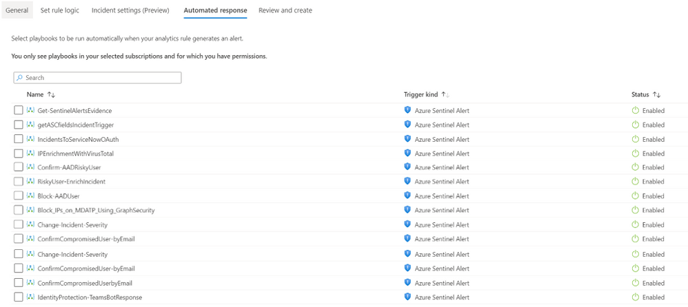
- Navigate to Azure Sentinel -> Analytics
- Create or Edit an existing schedule query rule
- Go to Automated response tab
- Select the multiple playbooks you would like to trigger.

It’s as simple as that!
At this point, the selected rules will run in no particular order. We are working on a new automation experience which will allow defining the order of execution as well – stay tuned.

by Contributed | Nov 9, 2020 | Technology
This article is contributed. See the original author and article here.
GPS has become part of our daily life. GPS is in cars for navigation, in smartphones helping us to find places, and more recently GPS has been helping us to avoid getting infected by COVID-19. Managing and analyzing mobility tracks is the core of my work. My group in Université libre de Bruxelles specializes in mobility data management. We build an open source database system for spatiotemporal trajectories, called MobilityDB. MobilityDB adds support for temporal and spatio-temporal objects to the Postgres database and its spatial extension, PostGIS. If you’re not yet familiar with spatiotemporal trajectories, not to worry, we’ll walk through some movement trajectories for a public transport bus in just a bit.
One of my team’s projects is to develop a distributed version of MobilityDB. This is where we came in touch with the Citus extension to Postgres and the Citus engineering team. This post presents issues and solutions for distributed query processing of movement trajectory data. GPS is the most common source of trajectory data, but the ideas in this post also apply to movement trajectories collected by other location tracking sensors, such as radar systems for aircraft, and AIS systems for sea vessels.

As a start, let’s explore the main concepts of trajectory data management, so you can see how to analyze geospatial movement trajectories.
The following animated gif shows a geospatial trajectory of a public transport bus1 that goes nearby an advertising billboard. What if you wanted to assess the visibility of the billboard to the passengers in the bus? If you can do this for all billboards and vehicles, then you would be able to extract interesting insights for advertising agencies to price the billboards, and for advertisers who are looking to optimize their campaigns.
 Throughout this post, I’ll use maps to visualize bus trajectories and advertising billboards in Brussels, so you can learn how to query where (and for how long) the advertising billboards are visible to the bus passengers. The background maps are courtesy of OpenStreetMap.
In the animated gif above, we simply assume that if the bus is within 30 meters to the billboard, then it is visible to its passengers. This “visibility” is indicated in the animation by the yellow flash around the billboard when the bus is within 30 meters of the billboard.
How to measure the billboard’s visibility to a moving bus using a database query?
Let’s prepare a toy PostGIS database that minimally represents the example in the previous animated gif—and then gradually develop an SQL query to assess the billboard visibility to the passengers in a moving bus.
If you are not familiar with PostGIS, it is probably the most popular extension to Postgres and is used for storing and querying spatial data. For the sake of this post, all you need to know is that PostGIS extends Postgres with data types for geometry point, line, and polygon. PostGIS also defines functions to measure the distance between geographic features and to test topological relationships such as intersection.
In the SQL code block below, first you create the PostGIS extension. And then you will create two tables: gpsPoint and billboard.
CREATE EXTENSION PostGIS;
CREATE TABLE gpsPoint (tripID int, pointID int, t timestamp, geom geometry(Point, 3812));
CREATE TABLE billboard(billboardID int, geom geometry(Point, 3812));

INSERT INTO gpsPoint Values
(1, 1, '2020-04-21 08:37:27', 'SRID=3812;POINT(651096.993815166 667028.114604598)'),
(1, 2, '2020-04-21 08:37:39', 'SRID=3812;POINT(651080.424535144 667123.352304597)'),
(1, 3, '2020-04-21 08:38:06', 'SRID=3812;POINT(651067.607438095 667173.570340437)'),
(1, 4, '2020-04-21 08:38:31', 'SRID=3812;POINT(651052.741845233 667213.026797244)'),
(1, 5, '2020-04-21 08:38:49', 'SRID=3812;POINT(651029.676773636 667255.556944161)'),
(1, 6, '2020-04-21 08:39:08', 'SRID=3812;POINT(651018.401101238 667271.441380755)'),
(2, 1, '2020-04-21 08:39:29', 'SRID=3812;POINT(651262.17004873  667119.331513367)'),
(2, 2, '2020-04-21 08:38:36', 'SRID=3812;POINT(651201.431447782 667089.682115196)'),
(2, 3, '2020-04-21 08:38:43', 'SRID=3812;POINT(651186.853162155 667091.138189286)'),
(2, 4, '2020-04-21 08:38:49', 'SRID=3812;POINT(651181.995412783 667077.531372716)'),
(2, 5, '2020-04-21 08:38:56', 'SRID=3812;POINT(651101.820139904 667041.076539663)');

INSERT INTO billboard Values
(1, 'SRID=3812;POINT(651066.289442793 667213.589577551)'),
(2, 'SRID=3812;POINT(651110.505092035 667166.698041233)');
The database is visualized in the map below. You can see that the gpsPoint table has points of two bus trips, trip 1 in blue and trip 2 in red. In the table, each point has a timestamp. The two billboards are the gray diamonds in the map.

Your next step is to find the locations where a bus is within 30 meters from a billboard—and also the durations, i.e., how long the moving bus is within 30 meters of the billboard.
SELECT tripID, pointID, billboardID
FROM gpsPoint a, billboard b
WHERE st_dwithin(a.geom, b.geom, 30);

--1    4    1
This PostGIS query above does not solve the problem. Yes, the condition in the WHERE clause finds the GPS points that are within 30 meters from a billboard. But the PostGIS query does not tell the duration of this event.
Furthermore, imagine that point 4 in trip 1 (the blue trip) was not given. This query would have then returned null. The problem with this query is that it does not deal with the continuity of the bus trip, i.e. the query does not deal with the movement trajectory of the bus.
We need to reconstruct a continuous movement trajectory out of the given GPS points. Below is another PostGIS query that would find both the locations of the billboard’s visibility to the passengers in the bus, and also the duration of how long the billboard was visible to the bus passengers.
1   WITH pointPair AS(
2     SELECT tripID, pointID AS p1, t AS t1, geom AS geom1,
3       lead(pointID, 1) OVER (PARTITION BY tripID ORDER BY pointID) p2,
4       lead(t, 1) OVER (PARTITION BY tripID ORDER BY pointID) t2,
5       lead(geom, 1) OVER (PARTITION BY tripID ORDER BY pointID) geom2
6     FROM gpsPoint
7   ), segment AS(
8     SELECT tripID, p1, p2, t1, t2,
9       st_makeline(geom1, geom2) geom
10    FROM pointPair
11    WHERE p2 IS NOT NULL
12  ), approach AS(
13    SELECT tripID, p1, p2, t1, t2, a.geom,
14      st_intersection(a.geom, st_exteriorRing(st_buffer(b.geom, 30))) visibilityTogglePoint
15    FROM segment a, billboard b
16    WHERE st_dwithin(a.geom, b.geom, 30)
17  )
18  SELECT tripID, p1, p2, t1, t2, geom, visibilityTogglePoint,
19    (st_lineLocatePoint(geom, visibilityTogglePoint) * (t2 - t1)) + t1 visibilityToggleTime
20  FROM approach;
Yes, the above PostGIS query is a rather complex one. We split the query into multiple common table expressions CTEs, to make it readable. In Postgres, CTEs give you the ability to “name” a subquery, to make it easier to write SQL queries consisting of multiple steps.
- The first CTE,
pointPair in Lines 1-7, uses the window function lead, in order to pack every pair of consecutive points, that belong to the same bus trip, into one tuple.
- This is a preparation for the second CTE,
segment in Lines 7-12, which then connects the two points with a line segment. This step can be seen as a linear interpolation of the path between every two GPS points.
The result of these two CTEs can be visualized in the map below:

Then the third CTE, approach Lines 12-18, finds the locations where the bus starts/ends to be within 30 meters from the billboard. This is done by drawing a circular ring with 30 meters diameter around the billboard, and intersecting it with the segments of the bus trajectory. We thus get the two points in the map below, marked with the black cross.

The last step in the earlier PostGIS query, Lines 19-22, computes the time at these two points using linear referencing, that is assuming a constant speed per segment2.

Exercise: try to find a simpler way to express the PostGIS query displayed earlier. I couldn’t. :)
The PostGIS query had to be that complex, because it programs two non-trivial concepts:
- Continuous movement trajectory: while the GPS data is discrete, we had to reconstruct the continuous movement trajectory.
- Spatiotemporal proximity: the continuous movement trajectory was used to find the location and time (i.e., spatiotemporal) during which the bus was within 30 meters from the billboard.
The good news for you is that MobilityDB can help make it easier to analyze these types of movement trajectories. MobilityDB is an extension of PostgreSQL and PostGIS that has implemented these spatiotemporal concepts as custom types and functions in Postgres.
MobilityDB: a moving object database system for Postgres & PostGIS
Let’s have a look on how to express this PostGIS query more simply using MobilityDB. Here is how the previous PostGIS query would be expressed in MobilityDB.
SELECT astext(atperiodset(trip, getTime(atValue(tdwithin(a.trip, b.geom, 30), TRUE))))
FROM busTrip a, billboard b
WHERE dwithin(a.trip, b.geom, 30)

--{[POINT(651063.737915354 667183.840879818)@2020-04-21 08:38:12.507515+02,
--  POINT(651052.741845233 667213.026797244)@2020-04-21 08:38:31+02,
--  POINT(651042.581085347 667231.762425657)@2020-04-21 08:38:38.929465+02]}
What you need to know about the MobilityDB query above:
- The table
busTrip has the attribute trip of type tgeompoint. It is the MobilityDB type for storing a complete trajectory.
- The nesting of
tdwithin->atValue->getTime will return the time periods during which a bus trip has been within a distance of 30 meters to a billboard.
- The function
atperiodset will restrict the bus trip to only these time periods.
- The function
astext converts the coordinates in the output to textual format.
- Accordingly, the result shows the part of the bus trip that starts at 2020-04-21 08:38:12.507515+02 and ends at 08:38:38.929465+02.
The MobilityDB documentation describes all of MobilityDB’s operations.
Now we step back, and show the creation of the busTrip table.
CREATE EXTENSION MobilityDB CASCADE;

CREATE TABLE busTrip(tripID, trip) AS
  SELECT tripID,tgeompointseq(array_agg(tgeompointinst(geom, t) ORDER BY t))
FROM gpsPoint
GROUP BY tripID;

--SELECT 2
--Query returned successfully in 78 msec.


SELECT tripID, astext(trip) FROM busTrip;

1  "[POINT(651096.993815166 667028.114604598)@2020-04-21 08:37:27+02,
       POINT(651080.424535144 667123.352304597)@2020-04-21 08:37:39+02,
       POINT(651067.607438095 667173.570340437)@2020-04-21 08:38:06+02,
       POINT(651052.741845233 667213.026797244)@2020-04-21 08:38:31+02,
       POINT(651029.676773636 667255.556944161)@2020-04-21 08:38:49+02,
       POINT(651018.401101238 667271.441380755)@2020-04-21 08:39:08+02]"
2  "[POINT(651201.431447782 667089.682115196)@2020-04-21 08:38:36+02,
       POINT(651186.853162155 667091.138189286)@2020-04-21 08:38:43+02,
       POINT(651181.995412783 667077.531372716)@2020-04-21 08:38:49+02,
       POINT(651101.820139904 667041.076539663)@2020-04-21 08:38:56+02,
       POINT(651262.17004873  667119.331513367)@2020-04-21 08:39:29+02]"
- The first step above is to create the MobilityDB extension in the database. In Postgres, the
CASCADE option results in executing the same statement on all the dependencies. In the query above—because PostGIS is a dependency of MobilityDB—CASCADE will also create the PostGIS extension, if it has not yet been created.
- The second query above creates the
busTrip table with two attributes (tripID int, trip tgeompoint). tgeompoint is the MobilityDB type to represent a movement trajectory. The tgeompoint attribute is constructed from a temporally sorted array of instants, each of which is a pair of a spatial point and a timestamp. This construction is expressed in the query above by the nesting of tgeompointinst -> array_agg -> tgeompointseq.
- The last
SELECT query above shows that the busTrip table contains two tuples, corresponding to the two trips. Every trip has the format [point1@time1, point2@time2, …].
Bigger than an elephant: how to query movement trajectories at scale, when a single Postgres node won’t do
As we now have two working solutions for measuring the billboard visibility: one in PostGIS and another one in MobilityDB, the next natural move is to apply these solutions to a big database of all bus trips in Brussels in the last year, and all billboards in Brussels. This amounts to roughly 5 million bus trips (roughly 5 billion GPS points) and a few thousand billboards. This size goes beyond what a single Postgres node can handle. Hence, we need to distribute the Postgres database.
This is a job for Citus, the extension to Postgres that transforms Postgres into a distributed database. Efficiently distributing the complex PostGIS query with many CTEs is a challenge we’ll leave to the Citus engineering team.
What I want to discuss here is the distribution of the MobilityDB query. Citus does not know the types and operations of MobilityDB. So the distribution is limited by what Citus can do in general for custom types and functions. My colleague, Mohamed Bakli, has done this assessment and published it in a paper titled “Distributed moving object data management in MobilityDB” in the ACM BigSpatial workshop (preprint) and in a demo paper titled “Distributed Mobility Data Management in MobilityDB” in the IEEE MDM conference (preprint).
The papers presented a solution to distribute MobilityDB using Citus. All the nodes in the Citus database cluster had PostgreSQL, PostGIS, MobilityDB, and Citus installed. The goal was to assess to what extent the spatiotemporal functions in MobilityDB can be distributed.
To do this assessment, the BerlinMOD benchmark (a tool for comparing moving object databases) was used. BerlinMOD consists of a trajectory data generator, and 17 benchmark queries that assess the features of a moving object database system. It was possible to execute 13 of the 17 BerlinMOD benchmark queries on a MobilityDB database cluster that is managed by Citus, without special customization.
See also the illuminating blog post about using custom types with Citus & Postgres, by Nils Dijk.
Back to our MobilityDB billboard visibility query, our mission is to calculate the billboard visibility for all billboards and all common transport vehicles in Brussels for an entire year.
We had set up a Citus database cluster, and created the MobilityDB extension in all its nodes. Then we used the Citus `create_distributed_table` function to distribute the busTrip table across all the worker nodes in the Citus database cluster. Next we made the billboard table a Citus reference table, and copied the reference table to all the worker nodes.
Here is the resulting distributed query plan:
EXPLAIN
SELECT atperiodset(trip, getTime(atValue(tdwithin(a.trip, b.geom, 30), TRUE)))
FROM busTrip a, billboard b
WHERE dwithin(a.trip, b.geom, 30);


Query plan
----------------------------------------------------------------------------------------
Custom Scan (Citus Adaptive)  (cost=0.00..0.00 rows=100000 width=32)
  Task Count: 32
  Tasks Shown: One of 32
  ->  Task
      Node: host=10.140.135.15 port=5432 dbname=roma
      ->  Nested Loop  (cost=0.14..41.75 rows=1 width=32)
          ->  Seq Scan on provinces_dist_102840 b (cost=0.00..7.15 rows=15 width=32)
          ->  Index Scan using spgist_bustrip_idx_102808 on bustrip_hash_tripid_102808 a
              (cost=0.14..2.30 rows=1 width=32)
              Index Cond: (trip && st_expand(b.geom, '30'::double precision))
              Filter: _dwithin(trip, b.geom, '30'::double precision)
The Citus distributed query executor parallelizes the query over all workers in the Citus cluster. Every node also has the MobilityDB extension, which means we can use MobilityDB functions such as dwithin in the query and in the indexes. Here for example, we see that the SP-GiST index on the Citus worker is used to efficiently evaluate the WHERE dwithin(…) clause.
With this, we come to the end of this post. To sum up, this post has two main takeaways:
If you’re ever looking to analyze movement trajectories to understand the spatiotemporal interaction of things across space and time, you now have a few new (open source!) options in your Postgres and PostGIS toolbox:
- MobilityDB can help you to manage and analyze geospatial (e.g. GPS, radar) movement trajectories in PostgreSQL.
- MobilityDB + Citus open source work together out of the box, so you can analyze geospatial movement trajectories at scale, too. Just add the two Postgres extensions (along with PostGIS) into your Postgres database, and you are ready to manage big geospatial trajectory datasets.
Footnotes
- Curious about the source of this data? The trajectory is for line 71 in Brussels, when it goes in front of my university campus ULB Solbosch. The public transport company in Brussels publishes an open API, where all the trajectories of their vehicles can be probed https://opendata.stib-mivb.be. The billboard location was invented by me, and the background map comes from OpenStreetMap. ↩
- It remains to compute the visibility duration, i.e., the difference in seconds between the two timestamps, which can be done by another CTE and window functions. Not to further complicate the query, we skip this detail here. ↩
by Contributed | Nov 9, 2020 | Technology
This article is contributed. See the original author and article here.
Howdy folks!
I’m excited to share today some super cool new features for managing users’ authentication methods: a new experience for admins to manage users’ methods in Azure Portal, and a set of new APIs for managing FIDO2 security keys, Passwordless sign-in with the Microsoft Authenticator app, and more.
Michael McLaughlin, one of our Identity team program managers, is back with a new guest blog post with information about the new UX and APIs. If your organization uses Azure AD Connect to synchronize user phone numbers, this post contains important updates for you.
As always, we’d love to hear any feedback or suggestions you may have. Please let us know what you think in the comments below or on the Azure Active Directory (Azure AD) feedback forum.
Best Regards,
Alex Simons (Twitter: Alex_A_Simons)
Corporate Vice President Program Management
Microsoft Identity Division
————–
Hi everyone!
In April I told you about APIs for managing authentication phone numbers and passwords, and promised you more was coming. Here’s what we’ve been doing since then!
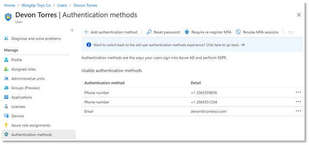
New User Authentication Methods UX
First, we have a new user experience in the Azure AD portal for managing users’ authentication methods. You can add, edit, and delete users’ authentication phone numbers and email addresses in this delightful experience, and, as we release new authentication methods over the coming months, they’ll all show up in this interface to be managed in one place. Even better, this new experience is built entirely on Microsoft Graph APIs so you can script all your authentication method management scenarios.

Updates to Authentication Phone Numbers
As part of our ongoing usability and security enhancements, we’ve also taken this opportunity to simplify how we handle phone numbers in Azure AD. Users now have two distinct sets of numbers:
- Public numbers, which are managed in the user profile and never used for authentication.
- Authentication numbers, which are managed in the new authentication methods blade and always kept private.
This new experience is now fully enabled for all cloud-only tenants and will be rolled out to Directory-synced tenants by May 1, 2021.
Importantly for Directory-synced tenants, this change will impact which phone numbers are used for authentication. Admins currently prepopulating users’ public numbers for MFA will need to update authentication numbers directly. Read about how to manage updates to your users’ authentication numbers here.
New Microsoft Graph APIs
In addition to all the above, we’ve released several new APIs to beta in Microsoft Graph! Using the authentication method APIs, you can now:
- Read and remove a user’s FIDO2 security keys
- Read and remove a user’s Passwordless Phone Sign-In capability with Microsoft Authenticator
- Read, add, update, and remove a user’s email address used for Self-Service Password Reset
We’ve also added new APIs to manage your authentication method policies for FIDO2 and Passwordless Microsoft Authenticator.
Here’s an example of calling GET all methods on a user with a FIDO2 security key:
Request:
GET https://graph.microsoft.com/beta/users/{{username}}/authentication/methods
Response:


We’re continuing to invest in the authentication methods APIs, and we encourage you to use them via Microsoft Graph or the Microsoft Graph PowerShell module for your authentication method sync and pre-registration needs. As we add more authentication methods to the APIs, you’ll be easily able to include those in your scripts too!
We have several more exciting additions and changes coming over the next few months, so stay tuned!
All the best,
Michael McLaughlin
Program Manager
Microsoft Identity Division
by Contributed | Nov 9, 2020 | Technology
This article is contributed. See the original author and article here.
I was working on this case where a customer load a certain amount of rows and when he compared the rows that he already had on the DW to the rows that he wanted to insert the process just get stuck for 2 hours and fails with TEMPDB full.
There was no transaction open or running before the query or even with the query. The query was running alone and failing alone.
This problem could be due to different reasons. I am just trying to show some possibilities to troubleshooting by writing this post.
Following some tips:
1) Check for transactions open that could fill your tempdb
2) Check if there is skew data causing a large amount of the data moving between the nodes (https://docs.microsoft.com/en-us/azure/synapse-analytics/sql-data-warehouse/sql-data-warehouse-tables-distribute#:~:text=A%20quick%20way%20to%20check%20for%20data%20skew,should%20be%20spread%20evenly%20across%20all%20the%20distributions.)
3) Check the stats. Maybe the plan is been misestimate. (https://docs.microsoft.com/en-us/azure/synapse-analytics/sql-data-warehouse/sql-data-warehouse-tables-statistics)
4)If like me, there was no skew data, no stats and no transaction open causing this.
So the next step was to check the select performance and execution plan.
1) Find the active queries:
SELECT *
FROM sys.dm_pdw_exec_requests
WHERE status not in ('Completed','Failed','Cancelled')
AND session_id <> session_id()
ORDER BY submit_time DESC;
2) By finding the query that you know is failing to get the query id:
SELECT * FROM sys.dm_pdw_request_steps
WHERE request_id = 'QID'
ORDER BY step_index;
3) Filter the step that is taking most of the time based on the last query results:
SELECT * FROM sys.dm_pdw_sql_requests
WHERE request_id = 'QID' AND step_index = XX;
4) From the last query results filter the distribution id and spid replace those values on the next query:
DBCC PDW_SHOWEXECUTIONPLAN ( distribution_id, spid )
We checked the XML plan that we got a sort to follow by estimated rows pretty high in each of the distributions. So it seems while the plan was been sorted in tempdb it just run out of space.
Hence, this was not a case of stats not updated and also the distribution keys were hashed as the same in all the tables involved which were temp tables.
If you want to know more:
https://docs.microsoft.com/en-us/azure/synapse-analytics/sql-data-warehouse/sql-data-warehouse-tables-distribute
https://techcommunity.microsoft.com/t5/datacat/choosing-hash-distributed-table-vs-round-robin-distributed-table/ba-p/305247
So basically we had something like:
SELECT TMP1.*
FROM    [#TMP1] AS TMP1
 LEFT OUTER JOIN [#TMP2] TMP2
     ON  TMP1.[key] = TMP2.[key]
 LEFT OUTER JOIN [#TMP3] TMP3
     ON  TMP1.[key] = TMP3.[key]
     AND TMP1.[Another_column] = TMP3.[Another_column]
 WHERE  TMP3.[key] IS NULL;
After we discussed we reach the conclusion what it was needed was everything from TMP1 that does not exist on TMP2 and TMP3. So as the plan with the LEFT Join was not a very good plan with a potential cartesian product we replace with the following:
SELECT TMP1.*
FROM    [#TMP1] AS TMP1
WHERE NOT EXISTS ( SELECT 1 FROM  [#TMP2] TMP2
                   WHERE TMP1.[key] = TMP2.[key])
 AND WHERE NOT EXISTS ( SELECT 1 FROM [#TMP3] TMP3
     WHERE TMP1.[key] = TMP3.[key] AND TMP1.[Another_column] = TMP3.[Another_column])
This second one runs in seconds. So the estimation was much better and the Tempdb was able to handle just fine.
That is it!
Liliam
UK Engineer.


.png")


.png")


Recent Comments