
by Contributed | Mar 10, 2023 | Technology
This article is contributed. See the original author and article here.
Hello hello, everyone! Happy Friday!
Here’s a recap of what’s been going on in the MTC this week.
MTC Moments of the Week
To start things off, we want to first give a huge shoutout to this week’s MTC Member of the Week – @Kidd_Ip! Kidd is a MCT (Microsoft Certified Trainer) and full time IT pro who has made great contributions to a variety of Tech Community forums across Azure and M365. Way to go, Kidd!
Moving to events, on Wednesday, we had our first of two AMA’s. Azure Communication Services and Microsoft Teams joined forces for this event to talk about the possibilities of connecting Teams with the communication capabilities in Azure and the cool stuff we can build with it. A big thank you to our speakers @MilanKaur, @tchladek, and @dayshacarter for sharing your expertise!
Then on Thursday, we had our second AMA all about Windows Server – from upgrading older versions and the importance of regular updates, to the security features in the latest versions of Windows Server (2022). We received a lot of questions, which were answered by our panel of speakers from the Windows Servicing and Delivery team as well as Windows Server engineers and security product managers. Shout out to @Artem Pronichkin , @Rick Claus, @Scottmca, @Ned Pyle, @Rob Hindman, and the rest team for a great session!
And over on the Blogs, in honor of Women’s History Month, the Marketplace Community kicked off a series of interviews with women leaders in the ISV community. The first edition of this series features an interview between @justinroyal and Harmke Alkemade, AI Cloud Solution Architect at Microsoft and Co-Founder at Friendly Flows. We love to see it!
Upcoming Events – Mark Your Calendars!
———-
For this week’s fun fact…
Did you know that the concept of what we know today as “Spring Break” (in the US, at least) began in 1938, when a college swimming coach, Sam Ingram, brought his team down from New York to Fort Lauderdale, Florida in 1936 to train? When the word got around to other swim coaches, they followed suit, and it began an annual pilgrimage for swimmers from across the US to enjoy the sun – and have some fun. The more you know!
Have a great weekend, everyone, and don’t forget to spring forward on Sunday!

by Contributed | Mar 10, 2023 | Technology
This article is contributed. See the original author and article here.
Welcome to the conclusion of our series on OpenAI and Microsoft Sentinel! Back in Part 1, we introduced the Azure Logic Apps connector for OpenAI and explored the parameters that influence text completion from the GPT3 family of OpenAI Large Language Models (LLMs) with a simple use case: describing the MITRE ATT&CK tactics associated with a Microsoft Sentinel incident. Part 2 covered another useful scenario, summarizing a KQL analytics rule extracted from Sentinel using its REST API. In Part 3, we revisited the first use case and compared the Text Completion (DaVinci) and Chat Completion (Turbo) models. What’s left to cover? Well, quite a lot – let’s get started!
There is some incredible work happening every day by Microsoft employees, MVPs, partners, and independent researchers to harness the power of generative AI everywhere. Within the security field, though, one of the most important topics for AI researchers is data privacy. We could easily extract all entities from a Microsoft Sentinel incident and send them through OpenAI’s API for ChatGPT to summarize and draw conclusions – in fact, I’ve seen half a dozen new projects on GitHub just this week doing exactly that. It’s certainly a fun project for development and testing, but no enterprise SOC wants to export potentially sensitive file hashes, IP addresses, domains, workstation hostnames, and security principals to a third party without strictly defined data sharing agreements (or at all, if they can help it). How can we keep sensitive information private to the organization while still getting benefit from innovative AI solutions such as ChatGPT?
Enter Azure OpenAI Service!
Azure OpenAI Service provides REST API access to the same GPT-3.5, Codex, DALL-E 2, and other LLMs that we worked with earlier in this series, but with the security and enterprise benefits of Microsoft Azure. This service is deployed within your Azure subscription with encryption of data at rest and data privacy governed by Microsoft’s Responsible AI principles. Text completion models including DaVinci have been generally available on Azure OpenAI Service since December 14, 2022. While this article was being written, ChatGPT powered by the gpt-3.5-turbo model was just added to Preview. Access is limited right now, so be sure to apply for access to Azure OpenAI!
ChatGPT on Azure solves a major challenge in operationalizing generative AI LLMs for use in an enterprise SOC. We’ve already seen automation for summarizing incident details, related entities, and analytic rules – and if you’ve followed this series, we’ve actually built several examples! What’s next? I’ve compiled a few examples that I think highlight where AI will bring the most value to a security team in the coming weeks and months.
- As an AI copilot for SOC analysts and incident responders, ChatGPT could power a natural language assistant interfacing with security operators through Microsoft Teams to provide a common operating picture of an incident in progress. Check out Chris Stelzer’s innovative work with #SOCGPT for an example of this capability.
- ChatGPT could give analysts a head start on hunting for advanced threats in Microsoft 365 Defender Advanced Hunting by transforming Sentinel analytic rules into product-specific hunting queries. A Microsoft colleague has done some pioneering work with ChatGPT for purple-teaming scenarios, both generating and detecting exploit code – the possibilities here are endless.
- ChatGPT’s ability to summarize large amounts of information could make it invaluable for incident documentation. Imagine an internal SharePoint with summaries on every closed incident from the past two years!
There are still a few areas where ChatGPT, as innovative as it is, won’t replace human expertise and purpose-built systems. Entity research is one such example; it’s absolutely crucial to have fully defined, normalized telemetry for security analytics and entity mapping. ChatGPT’s models are trained on a very large but still finite set of data and cannot be relied on for real-time threat intelligence. Similarly, ChatGPT’s generated code must always be reviewed before being implemented in production.
I can’t wait to see what happens with OpenAI and security research this year! What security use cases have you found for generative AI? Leave a comment below!
by Contributed | Mar 9, 2023 | Technology
This article is contributed. See the original author and article here.
Processing health insurance claims can be quite complex. This complexity is driven by a few factors, such as the messaging standards, the exchange protocol, workflow orchestration, all the way to the ingestion of the claim information in a standardize and scalable data stores. To enable operational, financial, and patient-centric data analytics, the claims data stores are often mapped to patient health records at the cohort, organization, or even population level.
What is X12 EDI?
Electronic Data Interchange (EDI) defines a messaging mechanism for unified communication across different organizations. X12 claims based processing refers to a set of standards for electronic data interchange (EDI) used in the healthcare industry to exchange information related to health claims. The X12 standard defines a specific format for electronic transactions that allows healthcare providers, insurers (payers), and other stakeholders to exchange data in a consistent and efficient manner. This cross-industry standard is accredited by the American National Standards Institution (ANSI). For simplicity, we will refer to ‘X12 EDI’ as ‘X12’ throughout this article.
What is FHIR?
FHIR® (Fast Healthcare Interoperability Resources) is a standard for exchanging information in the healthcare industry through web-based APIs with a broad range of resources to accommodate various healthcare use cases. These resources include patient demographics, clinical observations, medications, claims and procedures to name a few. It aims to improve the quality and efficiency of healthcare by promoting interoperability between different systems.
Azure Health Data Services is a suite of purpose-built technologies for protected health information (PHI) in the cloud. The FHIR service in Azure Health Data Services enables rapid exchange of health data using the Fast Healthcare Interoperability Resources (FHIR®) data standard. As part of a managed Platform-as-a-Service (PaaS), the FHIR service makes it easy for anyone working with health data to securely store and exchange Protected Health Information (PHI) in the cloud.
Why Convert X12 to FHIR?
FHIR is a modern, developer-friendly, born-in-the-cloud data standard compared to the aging X12. Converting from X12 to FHIR has many merits; (1) take advantage of FHIR interoperability and adoption to exchange claim information across various systems using modern and secure protocols, (2) unification of patient health and claim dataset into a single FHIR service in the cloud (3) enjoy a larger community of developers and evolving ecosystem at the global healthcare stage.
The Azure Solution
In essence, this article describes how to orchestrate the conversion of X12 claims to FHIR messages using Azure FHIR Service (with Azure Health Data Services), Azure Integration Account and Azure Logic Apps. Azure Logic Apps is a service within the Azure platform that enables developers to create workflows and automate business processes through the use of low-code/no-code visual and integration-based connectors. The service allows you to create, schedule, and manage workflows, that can be triggered by various events, such as receiving an HTTPS request or the arrival of a new file in an SFTP service. The Azure Integration Account is part of the Logic Apps Enterprise Integration Pack (EIP) and is a secure, manageable and scalable container for the integration artifacts that you create. The X12 XML Schema will be provided through the Azure Integration Account. The complete implementation of the X12 to FHIR conversion in Azure is available on GitHub.
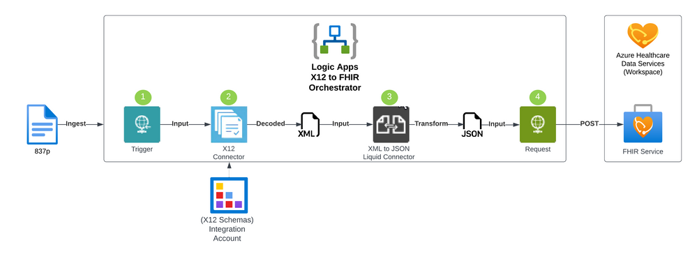
Orchestration of X12 to FHIR Conversion
Azure Logic Apps orchestrates the conversion process from X12 to FHIR resources, allows for additional data quality checks, and then ingests the FHIR resources in the Azure FHIR Service as depicted in the following 4 steps:
X12 to FHIR
- First, we ingest the X12 file content into the Azure Logic Apps workflow. In this sample, we submit the X12 file content in the body of an HTTPS Post request to the HTTPS endpoint exposed by Azure Logic Apps.
- Initial data quality check and decoding is done using the Azure Logic Apps X12 connector leveraging the X12 XML schemas associated with the transaction sets. This step will verify that the sender is configured and enabled in the system and pick the correct agreement that is configured with the X12 schema. This schema is used to convert the X12 data to XML.
- Once the X12 file is validated and decoded into the XML format, the XML content can then be converted to FHIR using the Azure Logic Apps XML to JSON Liquid connector. This uses DotLiquid templates to map the XML content to the corresponding FHIR resources.
- The output of the workflow is to store the data in Azure FHIR Service (with Azure Health Data Services) to support a unified view of the patient’s record. The FHIR service supports an HTTP REST endpoint where individual resources can be managed or sent as an atomic transaction using a FHIR bundle.
FHIR Resources
Various FHIR resources can be generated from an X12 transaction set. Depending on business requirements and entities participating in the integration, these resources will vary.
Entity |
Resource |
Description |
Patient |
Patient |
The person who the claim is for. |
Sender |
Organization or Practitioner |
The organization or provider submitting the claim. |
Recipient |
Organization or Practitioner |
The organization or provider receiving the claim for processing. |
Claim |
Claim |
The details about the services, amounts, and codes associated with the claim. |
Transaction Set / Message |
Communication |
Metadata bout the X12 message including the raw message. |
Liquid Template Sample
A sample liquid template is provided showing how to extract data from the decoded X12 file. In the following snippet, the elements under ‘content’ correspond to XML elements in the decoded X12 file. The XML elements are being mapped to the ‘total’ attribute of the ‘Claim’ FHIR resource.
{
    "resourceType": "Claim",
    "status": "active",
    "use": "claim",
    "total": "{{content.FunctionalGroup.TransactionSet.X12_00501_835.TS835_2000_Loop.TS835_2100_Loop.CLP_ClaimPaymentInformation.CLP03_TotalClaimChargeAmount}}"
}
Considerations
- Patient and provider identifiers in the transaction set may not correspond directly to the FHIR identifiers for those matching resources. A lookup approach may be needed to map the data such as an EMPI (enterprise master patient index) and Provider Registry. These mappings can exist in a separate data store or using the FHIR Identifier data type for the corresponding FHIR resource.
- Various X12 EDI schemas may need to be managed across your provider base. Each version of the transaction set will have a corresponding Liquid template which will also need to be versioned to convert the correct XML to FHIR. An approach around modularizing templates will be crucial to find the right balance for reusability.
- Depending on the scale of the provider base and security requirements the architecture can be revised accordingly:
- One instance of Azure Logic Apps can be created per provider providing full compute isolation.
- Azure Logic Apps also support parallelization allowing for a batch of X12 files to be submitted and then processed in parallel.
- One instance of Azure Logic Apps and Azure FHIR Service can be associated with a certain geographic region which may be needed if data sovereignty is required.
- Depending on business scenario, the ingestion process can be trigger from an SFTP event. Health organizations and providers can be associated with an Azure Storage Account enabled with SFTP where they can securely connect and manage their X12 artifacts.
References
by Contributed | Mar 8, 2023 | Technology
This article is contributed. See the original author and article here.
Start monitoring Delivery Optimization usage and performance across your organization today! Following the Windows Update for Business reports announcement back in November 2022, we are excited to announce the general availability of the Delivery Optimization Windows Update for Business report.
We genuinely appreciate those of you who participated in the public preview! You helped us verify the accuracy of the new data tables and revise the layout. Your responses helped us identify and address all critical issues, so it can now be offered to all Delivery Optimization users. In this article, find guidance to:
- Get started with Windows Update for Business reports
- Customize your Delivery Optimization report
Get started with Windows Update for Business reports
If you’re an existing Update Compliance user, you’re probably aware of the Update Compliance migration to Windows Update for Business reports. The new report experience provides templates for Windows reporting for monitoring organization and device level data with the added flexibility to customize a given report.
The Delivery Optimization Window Update for Business report provides a familiar experience, surfacing important data points that supply a unified way to check the performance across your organization. It contains data for the last 28 days, and we’ve added the long-awaited Microsoft Connected Cache data. In addition, we’ve reorganized the information to be more easily discoverable, leveraging the key cards that provide a quick and easy view of Delivery Optimization usage and performance.
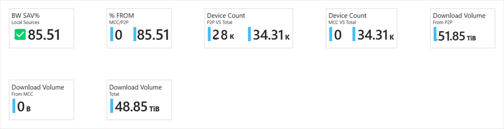
Key cards with main metrics in Windows Update for Business reports
You can quickly find the key pieces of data at the top of the report. We’ve bubbled up the metrics you care most about. You’ll find total bandwidth savings for both Delivery Optimization technologies, including peer-to-peer (P2P) and Connected Cache.
Further down the report, there are now three tabs that distinguish between Device configuration, Configuration details, and Efficiency by group.
Within Device configuration, you’ll see the breakdown of Download Mode configuration for your devices. Each configuration number in parentheses references the Download Mode set on the device.
 Device configuration details for peering status are shown as a pie chart while configuration names and device counts are shown as a bar graph in Windows Update for Business reports
In Content distribution, you can explore the breakdown of how bytes are delivered, from CDN/HTTP source, peers, or Connected Cache. You can also visualize the delivery method based on the different content types. By clicking on a particular content type, further drill down to richer content type details.
See an example of a particular environment that does not have an Connected Cache cache server, displaying 0% of bytes.
 Content distribution is visualized as a pie chart broken down by source type and a bar graph of volume by content type and source
The last tab presents a new option. Most of your organizations use policies to create peering groups to manage devices. In the Efficiency by group section, you can toggle among four different options. After talking with many of you, we’ve generally seen that device groups for Delivery Optimization are managed in four common ways by:
We’ve added each of these as a quick and easy tab, so you can view the top 10 groups by number of devices. So, for example, if you’re looking at the GroupID, you’ll see the 10 top group IDs with the highest number of devices. Similarly, in the City or Country view, you’ll see the top 10 cities or countries with the greatest number of devices. Or perhaps you’re more interested in monitoring the top ISPs delivering content based on the number of devices within the organization – for that, we’ve included the ISP option.
 The Efficiency By Group tab shows the top 10 groups based on Group ID, along with pertinent details such as P2P percentage, volume, and device count
As mentioned above, this is just the start of a new offering that enables you to tailor your report to meet the requirements of your organization. We will continue to incorporate richer features and enhanced experience in the Delivery Optimization report based on your feedback.
Customize your Delivery Optimization report
Much of the excitement with this new report format is centered on flexibility. It’s easy to modify the report template to meet your needs or if you want to run queries to further investigate your data. To do this, you can use the Windows Updates for Business reports data schema where you can access the new Delivery Optimization-related schema tables:
See what these tables look like within the LogManagement section.
 The Microsoft Azure interface showing Logs options, focused on a list of tables, including UCClient, UCDOAggregateStatus, and U DOStatus
We recommend running a query on each table to learn of the available fields. Let’s take a brief look at each.
UCClient table
The UCClient table is used within the Delivery Optimization report to get OSBuild, OSBuildNumber, OSRevisionNumber, and OSFeatureStatus. The data from UCClient is joined with UCDOStatus to complete the Device configuration breakdown table. You’ll notice that in Edit mode, you can easily modify the query that builds this visualization. If any changes are needed, you can modify this query accordingly.
 The Azure Workbooks interface showing the DO Device Configuration breakdown in Edit mode
UCDOStatus table
One of the two tables that hold Delivery Optimization-only data is UCDOStatus. This table provides aggregated data on Delivery Optimization bandwidth utilization. Explore the data for a single device or by content type. For example, the ‘Peering Status’ pie chart is powered by the UCDOStatus table.
 The Peering Status pie chart, powered by the UCDOStatus table, is shown when editing the query item for DeviceCountPeering
UCDOAggregatedStatus table
The second Delivery Optimization-only data table is UCDOAggregatedStatus. The role of this table is twofold:
- Provide aggregates of all individual UCDOStatus records across the tenant.
- Summarize bandwidth savings across all devices enrolled with Delivery Optimization.
One way this table is used is to build the volume by content types. Similarly, this view can be easily changed either through the query or built-in UX controls available via Log Analytics.
 A bar graph summary of volume by content types, such as quality updates
Keep in touch
We hope you are as excited as we are about these new changes for Delivery Optimization reporting. There are many more things we plan to add in the future. If you have any feedback or feature requests, we’d love to hear from you! Please submit it using the Feedback link within the Azure portal.
 A feedback submission form inside the Microsoft Azure portal
Continue the conversation. Find best practices. Bookmark the Windows Tech Community and follow us @MSWindowsITPro on Twitter. Looking for support? Visit Windows on Microsoft Q&A.
by Contributed | Mar 7, 2023 | Technology
This article is contributed. See the original author and article here.
One of the most common pain points of scheduling online meetings, especially with people outside your organization, is the back-and-forth messages. Microsoft Bookings now makes it simple to avoid that back and forth, with Power Automate you can seamlessly integrate Webex with Bookings.
Together, Bookings and Webex, they provide a comprehensive solution for all your virtual meeting needs.
With Power Automate, the moment a booking is made on Microsoft Bookings, a Webex meeting is automatically scheduled with all the details of the booking, such as date, time, and attendees. No more back and forth emails or missed meetings due to double bookings.
An animated image demonstrating how to create a Webex meeting when a Microsoft Bookings appointment is created via a Power Automate template.
Don’t let scheduling virtual meetings stress you out anymore. With the integration of Microsoft Bookings, Webex, and Power Automate, you’ll be able to focus on what really matters – conducting successful and efficient virtual meetings. Upgrade your virtual meeting game today and experience seamless scheduling.

Recent Comments