by Contributed | May 25, 2021 | Technology
This article is contributed. See the original author and article here.
This year our winter season was one of the coldest I’ve ever experienced, bringing an array of winter related issues. One of the more costly winter issues I’ve seen are busted water faucets. I knew this was not something I wanted to face this year, so I started thinking about the preventable problem and a smarter solution than the traditional foam cover. After considering the design of a foam cover and its inability to fully protect against freezing temperatures, I constructed two insulated thermal units to cover each faucet of my home. Each unit contains an incandescent light to warm the surrounding surface wall of the water pipe connected to the faucet. To monitor effectiveness and alert of potential failures, I built an IoT based solution using an ESP8226 and Azure to monitor, store, and provide insight on the temperature from within the units.
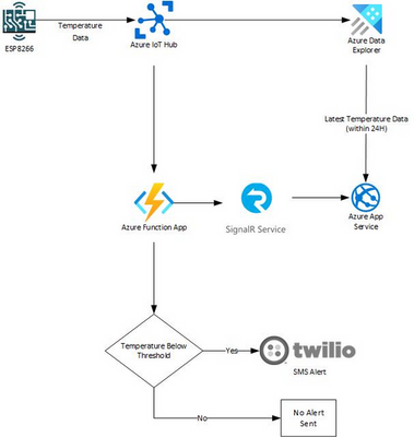
To keep this solution lean and efficient, I went with a serverless architecture and implemented Hot, Warm, and Cold data paths. This serverless architecture makes use of serverless resources in Azure, Functions, IoT Hub, Data Explorer, App Service, and Signal R, to ease the management and cost of the overall solution. To learn more about the power of serverless services and architectures on Azure, look here.
If you’re not familiar with Hot, Warm, and Cold data paths, take a look at the following breakdown to understand the differences between each path as well as which Azure services in this solution enable them:
Hot Path
- For processing or displaying data in real-time
- Real time alerting and streaming operations are performed using this data
- An Azure Function App, Signal R, and web app hosted on an Azure App Service are used here alert and stream data in real-time
- Azure Function App provides a consumption based and elastic resource to ingest all incoming data for processing, alerting, and sending to Azure Signal R
- Azure Signal R and the web app hosted on an Azure App Service enable the ability to stream data through a WebSocket based connection.
Warm Path
- For storing or displaying only a recent subset of data
- Small analytic and batch processing operations are performed on this data
- A web app hosted on an Azure App Service is used here as it can query and display the last 24 hours worth of temperature data per device from Azure Data Explorer
Cold Path
- For long-term storage of data
- Time consuming analytics and batch processing is performed on this data
- Azure Data Explorer is used here as it efficiently stores data for long periods of time, currently with a default of 100 years, and is an easy-to-use analytic engine, built on top of the Kusto Query Language (KQL)
Now each unit contains an ESP8266 with a DHT11 temperature sensor which can either send temperature data to my field gateway, IoT Edge running on a raspberry pi, or directly to Azure IoT Hub. This temperature data is then ingested, monitored, and displayed in real time using the following process:
- An Azure Data Explorer instance ingests all temperature data for long-term storage (Cold data path)
- An Azure Function broadcasts all temperature data to an Azure SignalR instance (Hot data path)
- This Azure Function also sends out a text alert if the temperature falls below a defined threshold
- The Azure SignalR instance broadcasts temperature data to all clients listening on a WebSocket based connection
- An App Service hosts a web app, displaying the latest temperature data record per device from the last 24 hours from Azure Data Explorer (Warm data Path)
- Finally, the web app creates a WebSocket connection to the Azure SignalR instance to receive temperature data in real time (Hot data path)
- If set up correctly, the web app will look like the following:

If you would like to recreate this solution, you can review my GitHub, link below, for instructions on how to set it up end-to-end.
https://github.com/niswitze/Hot-Warm-Cold-On-Azure-IoT
by Contributed | May 25, 2021 | Technology
This article is contributed. See the original author and article here.
Today, we are announcing a preview NuGet package, template, and Visual Studio v16.10 publishing support for creating OpenAPI enabled Azure Functions.
The OpenAPI Specification is an API description format for REST APIs and has become the leading convention for describing HTTP APIs. An OpenAPI description effectively describes your API surface; endpoints, operation parameters for each, authentication methods, and other metadata. As a part of the ecosystem already rich with tools and open-source packages for .NET, we wanted to extend this capability to Azure Functions.
In the early days of Azure Functions, there was a preview feature that allow you to use the OpenAPI specification to document your functions or endpoints. This feature experience was built into the Azure Portal, but never realized in the GA version of the product.
Brady Gaster showed the benefit of a well-designed API using ASP.NET Core and OpenAPI in this post on the ASP.NET Blog.
Getting Started
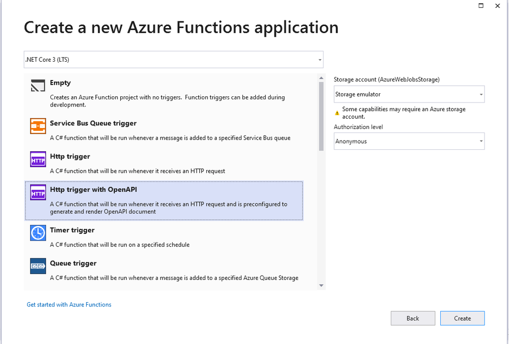
Using Visual Studio 16.10 or later, create a new Azure Functions project and choose the HttpTrigger template – “Http Trigger with OpenAPI”.

The new function is bootstrapped with the necessary implementation for OpenAPI support. When running the application, notice not only does the function emit the “Function1” endpoint as expected but also additional routes for a dynamic endpoint for OpenAPI document, Swagger document in JSON or YAML, Authentication redirects and the Swagger UI interactive app.

The additional routes are encapsulated when the function app is deployed, meaning that they are there but not exposed as public viewable routes.
Browsing to the `/api/swagger/ui` endpoint show the Swagger UI page which can be thought of as interactive documentation

The dynamic endpoint for the OpenAPI document accepts the version (v2 or v3) of the specification and the extension preferred (json or yaml). In the following example /api/openapi/v2.json returns the appropriate version of the specification in JSON. Note that the emitted JSON includes the operationId, an attribute used to provide a unique string-based identifier for each operation in the API. See more about generating HTTP API clients using Visual Studio Connected Services.

Publish and CI/CD support
As you can imagine, yes right click publish support is here for you. Using the known publishing dialog, pushing your OpenAPI enable function to AppService or Containers and provisioning the needed Azure resources are all handled.

Nothing has changed with the publishing of a new Azure Function, unless you want to also want to use this as a custom connector for your Power Apps. In Visual Studio 16.9 we added support for publishing to an existing Azure API Management service instances and creating new Consumption-mode instances of Azure API Management so you can use the monitoring, security, and integration capabilities of API Management.
In Visual Studio 16.10, the functionality is extended to support the Azure Function project that includes OpenAPI capabilities. When you are publishing an Azure Function with OpenAPI, the API Management tab allowing for selecting an existing instance or creating a new one.

Once the publish operation completes, you’ll be able to view and test the API operations within the API Management portal blade.
As an additional option, the provisioning and deployment of the Azure Function and related resources is now also available as a GitHub Action if your code in committed to a repository.

On finishing the publish dialog, a GitHub Action is created and committed to the repository triggered by a push of any change.

Using either method publishes or updates your Azure Function, creates or updates the API Management instance AND imports the function for you.
Azure API Management
Typically when adding a new API to the API Management instance you would have to manually define names, operations, parameters, endpoints and other metadata. When using the OpenAPI Extension, this is all done for you and any subsequent updates are also handled automatically. The following image shows the “Run” operation from the Azure Function along with all the configuration complete.

Add OpenAPI support to existing projects
For adding OpenAPI support to your existing Azure Functions, the Microsoft.Azure.WebJobs.Extensions.OpenApi package is available for .NET functions using the HttpTrigger. With just a few method decorators, the package makes your existing functions endpoints optimized for discovery.
public static class SayHello
{
    [FunctionName("SayHello")]
    [OpenApiOperation(operationId: "Run", tags: new[] { "name" })]
    [OpenApiParameter(name: "name", In = ParameterLocation.Query, Required = true, Type = typeof(string), Description = "Who do you want to say hello to?")]
    [OpenApiResponseWithBody(statusCode: HttpStatusCode.OK, contentType: "text/plain", bodyType: typeof(string), Description = "The OK response")]
    public static async Task<IActionResult> Run(
        [HttpTrigger(AuthorizationLevel.Anonymous, "get", "post", Route = null)] HttpRequest req,
        ILogger log)
    {
        log.LogInformation("C# HTTP trigger function processed a request.");
        string name = req.Query["name"];
        …
        return new OkObjectResult(responseMessage);
        }
    }
}
In this example, the AuthorizationLevel is set to “Anonymous”, however with the OpenApiSecurity decorator, using either “code” through querystring or “x-functions-key” through headers; additional security can be applied.
Summary
To learn more about the Azure Functions OpenAPI extension, visit the project on GitHub and checkout the preview documentation. As always. We’re interested in your feedback, please comment below and/or provide more in the issues tab on the repository.
We can’t wait to see what you build.
by Contributed | May 25, 2021 | Technology
This article is contributed. See the original author and article here.
Autodesk is popular for engineering classes in both universities and K-12 schools. We recently published a new class type that that shows how to set up a lab with Inventor and Revit for 3D design.
This class type includes the following information:
- Recommended VM size for the lab.
- How to setup Autodesk, including the licensing server.
- Example costing for the class.
Here is where you can find the new Autodesk class type: Set up a lab with Autodesk using Azure Lab Services – Azure Lab Services | Microsoft Docs
To see how Autodesk can be set up in a lab for Project Lead the Way, read the following class type: Set up Project Lead The Way labs with Azure Lab Services – Azure Lab Services | Microsoft Docs
Thanks!
Azure Lab Services team

by Scott Muniz | May 25, 2021 | Security, Technology
This article is contributed. See the original author and article here.
Official websites use .gov
A .gov website belongs to an official government organization in the United States.

Secure .gov websites use HTTPS A
lock ( )
) or
https:// means you’ve safely connected to the .gov website. Share sensitive information only on official, secure websites.
by Contributed | May 25, 2021 | Technology
This article is contributed. See the original author and article here.
In this installment of the weekly discussion revolving around the latest news and topics on Microsoft 365, hosts – Vesa Juvonen (Microsoft) | @vesajuvonen, Waldek Mastykarz (Microsoft) | @waldekm are joined by US-based, Microsoft Senior Product Designer on the SharePoint Team, Katie Swanson (Microsoft) | @kswansondesign. Topics discussed in this session include: The art of the possible, the design process and baking in customer feedback, accessibility testing, evolution of and possible future updates to SharePoint look book, diversity and inclusion in the PnP community and in IT generally. Microsoft and the Community delivered 16 articles in the last week!
Please remember to keep on providing us feedback on how we can help on this journey. We always welcome feedback on making the community more inclusive and diverse.
This episode was recorded on Monday, May 24, 2021.
These videos and podcasts are published each week and are intended to be roughly 45 – 60 minutes in length. Please do give us feedback on this video and podcast series and also do let us know if you have done something cool/useful so that we can cover that in the next weekly summary! The easiest way to let us know is to share your work on Twitter and add the hashtag #PnPWeekly. We are always on the lookout for refreshingly new content. “Sharing is caring!”
Here are all the links and people mentioned in this recording. Thanks, everyone for your contributions to the community!
Events:
Microsoft articles:
Community articles:
Additional resources:
If you’d like to hear from a specific community member in an upcoming recording and/or have specific questions for Microsoft 365 engineering or visitors – please let us know. We will do our best to address your requests or questions.
“Sharing is caring!”
by Contributed | May 25, 2021 | Technology
This article is contributed. See the original author and article here.
Hi all, Alan here again with a new article, I’m a Customer Engineer from Italy on Identity and Security.
In the past months I had several customers requesting about how to block sign-in from anonymous IP Addresses, one example would be someone using TOR Browser. So I thought this would help understand how to achieve this.
To do this we will use Azure AD “Conditional Access policy” with Session Control together with “Cloud App Security Conditional Access App Control”. Well yes sound the same but are quite different. Let’s see the details.
You will need access to you tenant’s Azure AD (portal.azure.com) and Cloud App Security (mycompany. portal.cloudappsecurity.com).
Thirst thing to do is create an Azure AD Conditional Access policy:
1. Navigate to your Azure Active Directory
2. Under Manage click on Security

3. Click on Conditional Access
4. Select New Policy

5. Give it a Name
6. Select to which users will apply
7. Select the cloud application, for this demo I will select Office 365

8. Go to Session and select Use Conditional Access App Control
9. Select Use Custom Policy

10. Click Select
11. Enable the policy and click Create

Once this is done the first time users log in Office 365 suite the application will be integrated in Cloud App Security
Open Cloud App Security portal : https://mycompany. portal.cloudappsecurity.com
On the top right side you have the configuration wheel, click and select “IP Address ranges” as shown below

One this interesting is that if you filter for one of the following Tags “Tor, Anonymous Proxy or Botnet” you will see it matches the following rule

So CAS has the “intelligence” to know which are these suspicious IP Addresses or networks
Here some more details Create anomaly detection policies in Cloud App Security | Microsoft Docs
- Activity from anonymous IP addresses
- Activity from suspicious IP addresses, Botnet C&C
- Activity from a TOR IP address
So back to our Connected Apps:
1. Go to Connected Apps

2. In the middle pane you will have three tabs, select “Conditional Access App Control apps”.
Below you will have a list of applications for which you can start creating CAS policies

3. Now browse to Control menu and select “Policies”

4. Select “ + Create policy”


5. The important part here is FILTERS and ACTIONS

6. Click on Create in order to create the policy and it will show it in the list

7. Access Office portal from the TOR Browser (use a valid user account from your Azure AD)

you will get the following error showing that you were blocked

Hope this article gives some hints on how to use Cloud App Security which I think is a great tool, simple and powerful and can really help enhance your security posture.
Have a good read :
Alan @CE
Customer Engineer – Microsoft Italy
by Contributed | May 25, 2021 | Technology
This article is contributed. See the original author and article here.
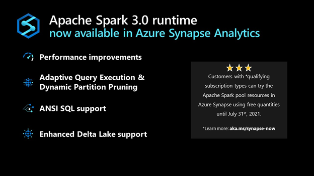
Starting today, the Apache Spark 3.0 runtime is now available in Azure Synapse. This version builds on top of existing open source and Microsoft specific enhancements to include additional unique improvements listed below. The combination of these enhancements results in a significantly faster processing capability than the open-source Spark 3.0.2 and 2.4.
The public preview announced today starts with the foundation based on the open-source Apache Spark 3.0 branch with subsequent updates leading up to a Generally Available version derived from the latest 3.1 branch.
Performance Improvements
In large-scale distributed systems, performance is never far from the top of mind, “to do more with the same” or “to do the same with less” are always key measures. In addition to the Azure Synapse performance improvements announced recently, Spark 3 brings new enhancements and the opportunity for the performance engineering team to do even more great work.
Predicate Pushdown and more efficient Shuffle Management build on the common performance patterns/optimizations that are often included in releases. The Azure Synapse specific optimizations in these areas have been ported over to augment the enhancements that come with Spark 3.
Adaptive Query Execution (AQE)
There is an attribute of data processing jobs run by data-intensive platforms like Apache Spark that differentiates them from more traditional data processing systems like relational databases. It is the volume of data and subsequently the length of the job to process it. It’s not uncommon for queries/data processing steps to take hours or even days to run in Spark. This presents unique challenges and opportunities to take a different approach to optimize and access the data. Over several days the query plan shape can change as estimates of data volume, skew, cardinality, etc., are replaced with actual measurements.
Adaptive Query Execution (AQE) in Azure Synapse provides a framework for dynamic optimization that brings significant performance improvement to Spark workloads and gives valuable time back to data and performance engineering teams by automating manual tasks.
AQE assists with:
- Shuffle partition tuning: This is a major source of manual work data teams deal with today.
- Join strategy optimization: This requires human review today and deep knowledge of query optimization to tune the types of joins used based on actual rather than estimated data.
Dynamic Partition Pruning
One of the common optimizations in high-scale query processors is eliminating the reading of certain partitions, with the adage that the less you read, the faster you go. However, not all partition elimination can be done as part of query optimization; some require execution time optimization. This feature is so critical to the performance that we added a version of this to the Apache Spark 2.4 codebase used in Azure Synapse. This is also built into the Spark 3.0 runtime now available in Azure Synapse.
ANSI SQL
Over the last 25+ years, SQL has become and continues to be one of the de-facto languages for data processing; even when using languages such as Python, C#, R, Scala, these frequently just expose a SQL call interface or generate SQL code.
One of SQL’s challenges as a language, going back to its earliest days, has been the different implementations by different vendors being incompatible with each other (including Spark SQL). ANSI SQL is generally seen as the common definition across all implementations. Using ANSI SQL leads to supporting the least amount of rework and relearning; as part of Apache Spark 3, there has been a big push to improve the ANSI compatibility within Spark SQL.
With these changes in place in Azure Synapse, the majority of folks who are familiar with some variant of SQL will feel very comfortable and productive in the Spark 3 environment.
Pandas
While we tend to focus on high-scale algorithms and APIs when working on a platform like Apache Spark, it does not diminish the value of highly popular and heavily used local-only APIs like pandas. In fact, for some time, Spark has included support for User Defined Functions (UDF’s) which make it easier and more scalable to run these local only libraries rather than just running them in the driver process.
Given that ~70% of all API calls on Spark are Python, supporting the language APIs is critical to maximize existing skills. In Spark 3, the UDF capability has been upgraded to include a capability only available in newer versions of Python, type hints. When combined with a new UDF implementation, with support for new Pandas UDF APIs and types, this release supports existing skills in a more performant environment.
Accelerator aware scheduling
The sheer volume of data and the richness of required analysis have made ML a core workload for systems such as Apache Spark. While it has been possible to use GPUs together with Spark for some time, Spark 3 includes optimization in the scheduler, a core part of the system, brought in from the Hydrogen project to support more efficient use of (hardware) accelerators. For hardware-accelerated Spark workloads running in Azure Synapse, there has been deep collaboration with Nvidia to deliver specific optimizations on top of their hardware and some of their dedicated APIs for running GPUs in Spark.
Delta Lake
Delta Lake is one of the most popular projects that can be used to augment Apache Spark. Azure Synapse uses the Linux Foundation open-source implementation of Delta Lake. Unfortunately, when running on Spark 2.4, the highest version of Delta Lake that is supported is Delta Lake 0.6.1. By adding support for Spark 3, it means that newer versions of Delta Lake can be used with Azure Synapse. Currently, Azure Synapse is shipping with support for Linux Foundation Delta Lake 0.8.
The biggest enhancements in 0.8 versus 0.6.1 are primarily around the SQL language and some of the APIs. It is now possible to perform most DDL and DML operations without leaving the Spark SQL language/environment. In addition, there have been significant enhancements to the MERGE statement/API (one of the most powerful capabilities of Delta Lake) expanding scope and capability.
Get Started Today
Customers with *qualifying subscription types can now try the Apache Spark pool resources in Azure Synapse using free quantities until July 31st, 2021 (up to 120 free vCore-hours per month).

by Contributed | May 24, 2021 | Technology
This article is contributed. See the original author and article here.
PostgreSQL continues to be extremely popular and is leveraged for a variety of use cases, particularly for modern applications requiring feature rich enterprise database, high performance, and scale. Our commitment to developers is to make Microsoft Azure the best cloud for PostgreSQL by bringing together the community and Azure innovations to help you innovate faster while ensuring that your data is secure. This extends to ensuring you can enjoy these similar innovations anywhere with Arc enabled Postgres Hyperscale.
This week at Microsoft Build, we’re excited to announce new capabilities, offers, and features that make it easier and more cost effective for developers to get started with PostgreSQL and receive support for the latest community innovation on Azure!
Making it easier and more cost effective to get started with Azure Database for PostgreSQL
During Ignite 2020 we announced Azure Database for PostgreSQL Flexible Server (Preview) deployment. I called out that there is a better way, and it is our strong belief that developers never have to make the hard tradeoff between using a managed solution and self-hosting on IaaS just to get more control of their databases or save costs. Fast forward, it turns out that our belief continues to be validated. We’ve had an overwhelming response from developers sharing their excitement around the ease of development, high performance, and the ability to optimize development costs with burstable pricing and stop/start capability. Furthermore, the flexibility with zone-redundant high-availability, and custom maintenance windows has enabled our customers to run their mission critical applications with piece of mind.
Ruben Schreurs, Group Chief Product Officer at Ebiquity Plc shared how Flexible Server is supporting their performance and scale requirements of their media analysis application.
“Our Azure Database for PostgreSQL Flexible Server has delivered incredible performance improvements across our client clusters. It was easy to set up and the native environment on Linux VM, High Availability support and a radical increase in storage scalability sets us up for the next phase of growth as Azure power users.”
Today, we are excited to announce that we’re making it even easier and more cost effective for developers to get started by introducing a free, 12-month offer for our new Flexible Server (Preview) deployment option. You can take advantage of this offer to use Flexible Server to develop and test your applications and run small workloads in production for free. This offer will be available with an Azure Free Account starting June 15th, 2021 and it provides up to 750 hours of Azure Database for PostgreSQL – Flexible Server and 32GB of storage per month for the first 12 months.
Over the last few months, we’ve continued to invest in Flexible Server by bringing support for the PostgreSQL 13 and popular PostgreSQL extensions, including pglogical, pg_partman, and pg_cron, in addition to another 50+ extensions. So, you can build with new open-source innovations while leveraging the benefits of a fully managed, flexible PostgreSQL service on Azure.
You can also take advantage of a built-in PgBouncer, which provides a built-in connection pooler to optimize the number of your connections, as well as expanded security capabilities with Private DNS Zone, which allows you to create a custom domain name and resolution within the current VNET or any in-region peered VNET.
Whether you’re building a new application or migrating an existing one, it should be easier than ever to get started and ensure your data is highly available, performant, and secure at the lowest TCO. Look at this quick demo, which illustrates just how easy it is to connect your application to an instance of Azure Database for PostgreSQL.
 Postgres Flexible Server Demo
Bringing the best of PostgreSQL innovations to Azure Database for PostgreSQL – Hyperscale (Citus)
When developing modern, cloud native applications, it’s critical to ensure that your application can scale as it grows. With Azure Database for PostgreSQL – Hyperscale (Citus), you can leverage high-performance horizontal scaling to achieve near limitless scale. Hyperscale (Citus) enables this by scaling queries across multiple machines using sharding, which provides greater scale and performance.
HSL transit authority shared how they improved traffic monitoring with Azure Database for PostgreSQL – Hyperscale (Citus). Sami Räsänen, Product Owner and Team Lead said
“Along with much better performance, moving to Hyperscale has reduced operational costs by over 50 percent.”
We’re excited to expand our offering so that you can now shard Postgres on a single Hyperscale (Citus) node using the new Basic tier. This means that you can start small and cost-effectively while being ready to easily scale out your database horizontally as your application grows. Learn more about this in the blog post Sharding Postgres with Basic tier in Hyperscale (Citus), how why & when.
Azure Database for PostgreSQL Hyperscale (Citus) supports the latest release, Citus 10 extension in preview. In addition to bringing the ability to shard Hyperscale (Citus) on a single node using the Basic tier, we are also providing columnar storage, which allows you compress your PostgreSQL and Hyperscale (Citus) tables to reduce storage cost and speed up your analytical queries. Learn more about the features and functionality in the blog post New Postgres superpowers in Hyperscale (Citus) with Citus 10.
We’ve added support for PostgreSQL 13, which provides major enhancements including de-duplication of B-tree index entries, increased performance for queries using aggregates or partitioned tables, better query planning when using extended statistics, parallelized vacuuming of indexes, incremental sorting, and more.
There are two easy ways to get started with Citus 10 and Hyperscale (Citus):
- Leverage the Basic Tier as the best way to try Citus 10 in Hyperscale (Citus) managed service.
- Run Citus open source on your computer as a single Docker container. Not only is the single docker run command an easy way to try out Citus—it gives you functional parity between your local dev machine and using Citus in the cloud.
Building together with the community
Our approach is not only to build the best PostgreSQL on Azure, but also to be fully integrated with the open-source community and to contribute to that community. Our team at Microsoft is contributing innovation, code, and leadership into the global PostgreSQL open-source project. Our PostgreSQL experts have committed key capabilities to the upcoming PostgreSQL release, including significantly faster crash recovery and increased connection scalability.
In addition, we continue to make the most contributions to the open-source community on GitHub of any cloud vendor. Some of our notable contributions include the PostgreSQL extension for Visual Studio Code and the Azure Data Studio PostgreSQL extension. You can also use the Citus open-source extension, which to date has had over 1.7 million downloads by customers who use it to scale-out PostgreSQL into a distributed database.
Bringing Advanced Security Capabilities to PostgreSQL
We continue to invest in bringing the latest security and compliance features to PostgreSQL. And are excited to share that Azure Defender for Open-source Relational Database is now generally available, offering comprehensive security for PostgreSQL. Azure Defender constantly monitors your PostgreSQL servers for security threats and detects anomalous database activities indicating potential threats to PostgreSQL resources.
We recommend protecting production instances of PostgreSQL with Azure Defender as part of your overall security strategy.
Looking ahead
With Azure Database for PostgreSQL, we’re on a mission to provide greater flexibility and make your application development easier and more affordable. In upcoming months, we plan to extend our support to Terraform deployment and automation, expand into additional Azure regions, and look forward to the announcement of General Availability for Azure Database for PostgreSQL Flexible Server.
Take the time to learn more about our Azure Database for PostgreSQL managed service. If you’re interested in diving deeper, Flexible Server docs, Hyperscale (Citus) docs, are a great place to start. Lastly, do not miss out on taking advantage of the free 12-month offer. We remain curious about hearing how you plan to use Flexible Server and Hyperscale (Citus) deployment options to drive innovation to your business and applications. We’re always eager to get your feedback, so please reach out via email to Ask Azure DB for PostgreSQL.

by Contributed | May 24, 2021 | Technology
This article is contributed. See the original author and article here.
When we announced Azure Database for MySQL Flexible Server at Microsoft Ignite last year, we made a commitment to the developer community and our customers to provide simplified development experience, increased flexibility, and cost optimization controls, while preserving all the benefits of a managed service. I called out that there is a better way, and it is our strong belief that developers never have to make the hard tradeoff between using a managed solution and self-hosting on IaaS just to get more control of their databases or save costs.
Fast forward to today, it turns out that you share our belief! Thus far thousands of customers are using the Flexible Server deployment option and your feedback continues to shape our product strategy, prioritization, and roadmap. As we continue to innovate on your behalf, today we are excited to announce a free 12-month offer for Flexible Server, additional options for scaling IOPs, and the general availability of Azure Defender support for MySQL.
Customer response
I want to start by sharing some feedback from our customers and the impact of Flexible Server in tackling real world challenges. A common theme around these stories is a reminder about how important developer productivity, cost, and continuous availability is to our customers, especially as they tackle real life challenges head-on. We’re extremely grateful to be able to enable our customers to achieve their goals, and we’re thankful that we could play a small role towards their success.
“We are a group of volunteers working for a non-profit organization to configure/deploy Moodle on Azure for an online learning solution for our community, which was essential for us during and post COVID. Being a non-profit, we run on thin budgets and our traffic is unpredictable. Azure Database for MySQL Flexible Server Burstable SKU enabled us to develop and test the solution at a significantly lower cost. It provided us with the right blend of performance and cost allowing us to focus on solution without any operational overhead for us”
– Rahim L, Solution Architect
Below is feedback from customers whose mission it is to entertain millions of people with streaming services and Gaming solutions, 24×7. These solution patterns require continuous availability and high performance to serve users without interruption and to accomplish this at minimal cost. MySQL Flexible Server is enabling these customers to run mission critical applications efficiently and with piece of mind.
“Being South Asia’s largest music and audio streaming service, performance, scale and high availability of the MySQL Database is critical for us to provide the millions of our users with a great listening experience round the clock. Our major motivation to move to Azure Database for MySQL Flexible Server is to leverage its performance stability, zone redundant high availability, and managed maintenance window feature which will allow us to control and minimize the downtime caused by monthly patching to ensure we minimize the interruptions for our end users” 
– Ramesh Sudini, Head of Engineering at JioSaavn
“We have successfully gone through CBT for game title Time Defender in Japan on MySQL Flexible Server. We prefer MySQL for our games and performance, reliability and high availability of the MySQL server is very critical for us. We evaluated Azure Database for MySQL Flexible Server and it perfectly met our performance and reliability goals. We love the managed maintenance window feature which gives us flexibility to schedule our maintenance window in addition to zone redundant HA which enable to have high availability. As all features are proved, we will launch game with flexible server in CY21 Q3.”
– Peter Lee, Lead of Service Development Unit, Vespa Inc.
Today, I’m extremely excited to make application development with Azure Database for MySQL Flexible Server more affordable, more secure, and even simpler.
Free 12-month offer!
Beginning June 15, 2021, new Azure users can start to develop and deploy applications leveraging Azure Database for MySQL Flexible Server (Preview) by taking advantage of our 12-month free account offer. This offer will be available with an Azure Free Account and provides up to 750 hours of Azure Database for MySQL – Flexible Server and 32GB of storage per month for the first 12 months. The Azure free account offers access to many other Azure services such as Azure Kubernetes Services, Azure App Services, and Azure VMs, which you can use to develop, test, and run your application for free for 12 months.
Gain increased cost efficiency by scaling IOPs independent of storage
Database applications often need sufficient IOPs to optimally perform IO intensive workload tasks. Azure Database for MySQL Flexible Server now offers the ability to scale IOPs on-demand and independently of provisioned storage size, giving developers more freedom and control. If your workload requires more IOPs only for a few hours to run a nightly data load job, or just for a one-time migration to Azure Database for MySQL Flexible Server, you can now scale IOPs on-demand to increase the speed of the job, and then scale down IOPs to save costs without incurring database downtime. Users continue to have the flexibility to increase provisioned storage in 1 GB increments, which automatically provides an incremental 3 baseline IOPs.
 Ability to scale IOPs independent of storage with MySQL Flexible Server
Enjoy additional free IOPs
Beginning July 2021, we’re also increasing the free IOPs for the Flexible Server deployment option from 100 to 300 and raising the minimum allowed provisioned storage to 20GB. This will give our users access to more IOPs for improved performance for IO intensive workloads without additional costs.
After this change, your free IOPs available with provisioned storage size will increase as shown in the table below:
Currently |
Beginning July, 2021 |
100 + 3 * [Storage provisioned in GB] IOPs |
300 + 3 * [Storage provisioned in GB] IOPs |
For example, if you have provisioned 20GB of storage, you currently get 160 IOPs (100 + 3 * 20GB). After the July 2021 update, with 20GB of provisioned storage you will get 360 IOPS (300 + 3 * 20GB).
MySQL 8.0 now available in Flexible Server
Immediately after the Flexible Server (Preview) release, many of you requested that we prioritize support for the latest MySQL 8.0 version. I’m happy to share that the MySQL 8.0.21 release is now available on Flexible Server, so you can now enjoy all the service capabilities and start developing with MySQL 8.0 version.
Other major updates
In addition to the exciting announcements above, Azure Database for MySQL Flexible Server now also provides:
Announcing General Availability of Azure Defender for Open-source Relational Database
We also continue to invest in bringing the latest security and compliance features to MySQL. We’re excited to share that Azure Defender for Open-source Relational Database, which offers comprehensive security for MySQL, is now generally available. Azure Defender support for MySQL constantly monitors your servers for security threats and detects anomalous database activities that could indicate potential threats to Azure Database for MySQL.
With this announcement, you can now protect your open-source databases with Azure Defender, expanding and strengthening your protection across your entire database estate. We recommend protecting production MySQL servers with Azure Defender as part of your overall security strategy.
Looking ahead
With Azure Database for MySQL Flexible Server, we’re on a mission to provide greater flexibility and make your application development easier and more affordable. In upcoming months, we plan to extend our support to Terraform deployment and automation, expand into additional Azure regions, and look forward to the announcement of General Availability for Azure Database for MySQL Flexible Server. We’re always eager to hear about how you plan to use the new Flexible Server deployment option to drive innovation for your business and applications. Please continue to send in your valuable feedback by emailing us at Ask Azure DB for MySQL.
In the interim, please take the time to learn more about our Azure Database for MySQL managed service. If you’re interested in diving deeper, Flexible Server documentation is a great place to start. Lastly, be sure not to miss out on taking advantage of the free 12-month offer!
by Contributed | May 24, 2021 | Technology
This article is contributed. See the original author and article here.
Hello everyone, this is David Loder again, sporting Microsoft’s new Customer Engineer title, but still a Hybrid Identity engineer from Detroit. Over the past year I’ve seen an uptick in requests from customers looking to modernize their GALSync solution. Either they’re wanting to control use of SharePoint and Teams B2B capabilities or looking to enable a GALSync with a cloud-only organization. And they’re asking for assistance and guidance that I hope to provide today.
Before I get started on how Microsoft Identity Manger (MIM) 2016 can help provide the basis for a supported GALSync solution, I want to ensure everyone knows that Microsoft provides a managed service SaaS offering to help with any multi-tenant syncing scenarios. It’s called Active Directory Synchronization Service (ADSS) and does all the back-end tenant syncing automagically. The great benefit with ADSS is that it’s a fully supported solution. MIM as a product is fully supported, but as has always been the case, any customizations put into it are best-effort support. Reach out to your account team if you want more information about ADSS. Now on with the MIM discussion.
Historically, Microsoft has provided a supported GALSync solution in our on-premises sync engine, MIM. Documentation on the GALSync configuration was first provided back in the Microsoft Identity Integration Server (MIIS) 2003 timeframe. Additional documentation is available at the GALSync Resources Wiki. Despite its age, that guidance still holds true today. But it is limited to an Active Directory to Active Directory user to contact sync design.
Today, we offer the Microsoft Graph Connector. It provides the ability to connect to an Azure AD tenant, and to manage B2B invitations. However, it is not a drop-in replacement for GALSync. We can get there, but we need to fill in some missing components.
There are many scenarios that Graph Connector could satisfy, and they can get increasingly difficult. For this blog I’ll focus on the simplest scenario and then discuss what considerations one would have in order to move to more complex scenarios.
In a classic GALSync solution, we sync users from a partner AD to become contacts in our home AD. For this Azure AD replacement, we want to sync users from a partner tenant, and make them B2B users in our home tenant. This assumes that you’ve moved past the point where you need identical GALs in both on-premises Exchange and Exchange Online. Most of the customers I work with have gotten to that point. Maybe they still have some service account mailboxes left to move, but all humans who need to view a GAL have been moved to Exchange Online. That simplifies the requirements as there’s no longer a need for creating on-premises objects for Exchange to use.
The first component we need is MIM 2016. If you are an Azure AD Premium customer, MIM is still fully supported and still available for download. Otherwise, MIM is in extended support through 2026. To keep our infrastructure footprint small, this solution will use only a Sync Service install, and will not use the Portal or any declarative provisioning.
With a base MIM install in place we’re almost ready to make a Graph connection to our first tenant. But before we do so, we need to have a discussion of scope, because scope is the major factor in determining the complexity of solution. When talking about scope, I’m going to be very exact in terms of objects and attributes as much of our terminology in this space is vague and subject to perspective to understand meaning.
“We want users from a partner tenant….” Starting with this phrase, we need to break it down to a scoped object and attribute definition. The Graph Connector exposes user and contact (technically orgContact) object classes. We will only want to bring in users from the partner tenant. Except the user object class covers both internal and external (a.k.a. B2B) users. Typically, we only want to bring in the internal users from the partner tenant. We can tell the difference between them because external users have a creationType attribute equal to ‘Invitation’, whereas internal users have a null creationType. The other possible choice one might consider is the userType attribute with values of either ‘Guest’ or ‘Member’. But I think that is a poor choice. Internal users are Member by default and external users are Guest by default, but userType can be changed for both. Guest vs. Member only controls one’s default visibility to certain workloads such as SharePoint or Azure AD itself. Guest is sometimes incorrectly used interchangeably with B2B, but those two terms are not equivalent.
“Make B2B users in our home tenant….” Given the previous discussion, this phrase is now rather easy to scope. We’ll be looking at user objects with creationType=’Invitation’.
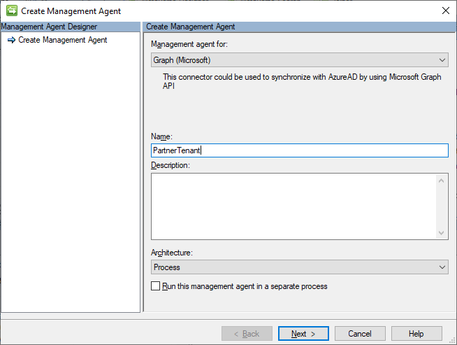
With our purposefully simplistic scope defined, let’s build the first Graph connection to the partner tenant. Install the Graph Connector on the MIM system. There have been lots of fixes recently so be sure to use the current version.
Start with creating a new Graph (Microsoft) connector.
Provide registered app credentials to connect to the partner tenant. The app registration needs at least User.Read.All and Directory.Read.All, with Admin consent. This is an example from one of my temporary demo tenants.

On the Schema 1 page, keep the Add objects filter unchecked. Unfortunately, we cannot use the filtering capability to return only the internal users where creationType is null. The Graph API provides more advanced filtering capabilities, but it requires a Header value to be set, which the Graph Connector does not currently expose as a configurable setting.
On the Select Object Types page check user.
On the Select Attributes page, let’s select a minimum number of attributes to enable decent GAL functionality as part of the B2B sync. Additional attributes can be added if the GAL needs to be more fully populated. Select creationType, displayName, givenName, id, mail, showInAddressList, and surname.

The anchor attribute on the Configure Anchors page will automatically be set to id.
On the Configure Connector Filter page, I will keep this example simple by using a declared filter of creationType Is present. This will filter out any external users that may happen to already exist in the partner tenant. But this filtering will come at the expense of increased Delta Sync times due to having to process each filtered disconnector every sync cycle.

For Configure Join and Projection Rules, we’ll join on id first, mail second, otherwise project as a person.

This is the inbound partner tenant user flow, so provide a direct inbound flow for each attribute. Several of the selected attributes are not default metaverse attributes, so the metaverse schema will need to be extended to account for these attributes.

Leave the Configure Deprovisioning page at the default of ‘Make them disconnectors’ and Configure Extensions page will also be left at its default of empty.
Create the Full Import and Full Sync run profiles. Execute them to confirm that the partner tenant users are projected into the metaverse. Also create the Delta Import and Delta Sync run profiles. We won’t use them now, but will need them later. I’ve gotten spoiled from AADC creating run profiles by default.
Now that the inbound side from the partner tenant is complete, let’s create the outbound side for the home tenant. The setup will be similar to the inbound side, but with some minor changes.
The App Registration in the home tenant will require the Directory.Read.All and User.ReadWrite.All permissions. There is a User.Invite.All permission, but since we need to sync GAL attributes after the invite, that permission does not provide enough access for this scenario.
For the Schema 1 page, we’ll need to leave the Add objects filter checkbox uncheck again. Even though we could technically set a graph filter of creationType eq ‘Invitation’, using a filter breaks Delta Imports for the Graph Connector (with a no-start-ma error). We will have to continue to use MIM filtering the keep the scope correct since Delta Imports are very important for most of my customers.
On the Global Parameters page set the Invite redirect URL to https://myapps.microsoft.com/?tenantid=GUIDValue. Leave the send mail checkbox unchecked unless you want to start automatically spamming all your invitees.

On the Select Attributes page, include userPrincipalName and userType in addition to the list of attributes from the inbound side. We’re selecting UPN just so we can see the full results of the invitation process, not because we’ll be doing any syncing of that attribute.
For the Configure Connector Filter page, we reverse it from the inbound partner tenant setting and use a filter of creationType Is not present.
On the Configure Join and Projection Rules page, only add the Join Rule for mail. There should be no Projection Rule as we want all the external users to project into the metaverse from the inbound partner tenant.
For the Configure Attribute Flow page, add a direct export (allowing nulls) for displayName, givenName, mail, showInAddressList and surname. Add a constant export of Guest for userType. While an external user is typically Guest by default, the Graph Connector defaults to Member, so we need to override that. Also add a constant export of Invitation for creationType. For the creationType, we’re flowing that just to satisfy the MA filter, not that it affects the invitation process.

On the Configure Deprovisioning page, change the selection to Stage a delete on the object for the next export run.
Create and run the Full Import and Full Sync run profiles. If there are any matching mail values for existing external users those should join. Otherwise, the existing external users will show up as disconnectors. Also create the Delta Import, Delta Sync and Export run profiles. We won’t use them now, but will need them later.
Finally, we need a small amount of provisioning code to provision the external users from the metaverse into the home tenant MA. From the Tools > Options… menu check the Enable metaverse rules extension checkbox. Then click the Create Rules Extension Project… button. I’ll provide sample code for Visual C#, so choose that selection and the version of Visual Studio to use to compile the project.
This is a sample implementation for the IMVSynchronization.Provision method.
void IMVSynchronization.Provision (MVEntry mventry)
{
string container = “OBJECT=user”;
string rdn = “CN=” + Guid.NewGuid().ToString();
ConnectedMA HomeTenantMA = mventry.ConnectedMAs[“HomeTenant”];
ReferenceValue dn = HomeTenantMA.EscapeDNComponent(rdn).Concat(container);
int numConnectors = HomeTenantMA.Connectors.Count;
// If there is no connector present, create a new connector.
if (numConnectors == 0)
{
CSEntry csentry = HomeTenantMA.Connectors.StartNewConnector(“user”);
csentry.DN = dn;
csentry[“id”].StringValue = Guid.NewGuid().ToString();
csentry.CommitNewConnector();
}
else if (numConnectors == 1)
{
//Do nothing, no rename is needed
}
else
{
throw (new UnexpectedDataException(“multiple connectors:” + numConnectors.ToString()));
}
}
A few things to note in this code. We need the name of the home tenant MA as the connected MA we are managing. We also set a random GUID-based DN and id in order to successfully export the invitation, but those values will be replaced by the real Azure AD values during the first confirming import.
Build the solution in Visual Studio and make sure the extension DLL gets copied to the Microsoft Forefront Identity Manager2010Synchronization ServiceExtensions folder. Back in the Options dialog, ensure the DLL that was just created is selected for the Rules extension name, and check the Enable Provisioning Rules Extension checkbox.

To begin with a small test, pick a sample user from the partner tenant MA and commit a Full Sync Preview against them. That should generate a pending export in the home tenant MA.

The small piece of magic with the Graph Connector is that if a user has a pending add with mail but no UPN, they will go through the invitation process to make them an external user, rather than being created as an internal user. We can see the pending export with the temporary DN and id, the GALSync attributes we wired up, and our constant userType of Guest. This test user has an OnMicrosoft.com mail address in the partner tenant as I have not added a custom domain to that tenant. The actual mail value is ultimately immaterial so long as it doesn’t already belong to the destination tenant.
Run the Export, followed by a confirming Delta Import.

We see that the user got successfully invited, got its real DN and id and has all the attributes we set. Notice the UPN got automatically set by AAD in the expected format of mail#EXT#@tenant. It also was given a default setting of showInAddressList = false. By default, invited external users are hidden from the GAL.
Complete a second delta sync cycle (Delta Import, Delta Sync, Export) and showInAddressList should get set to its synced value. For this example user, that would be a null value.

After exporting the updated showInAddressList value, we can confirm that our GALSync is functional. Log in to Outlook on the web in the home tenant, open the People app and select the All Users GAL. We should see our newly synced user present in the GAL.

Finally, to complete the deprovisioning aspect of the GALSync, configure the Object Deletion Rule for the person object class to delete the metaverse object when the partner tenant connector is disconnected. This way, a deletion of the user from the partner tenant will cascade a delete of the external B2B user to our home tenant.
That’s the end of the setup for GALSync from a single source to a single destination tenant.
As I alluded to at the beginning, more complex setups are possible. Consider a bi-directional GALSync where the partner tenant also needs the users from our home tenant. One way to keep the architecture simple is to maintain one MIM instance per tenant; we simply duplicate this setup in the opposite direction. This is identical to the AADC architecture where one AADC is needed for each tenant. It allows the provisioning code to know the tenant for which it is responsible, cleanly separates inbound from outbound flows and causes no precedence problems. It also allows the partner to control the app registration which possesses write access into their tenant.
Or consider a full-mesh setup where the tenants are all peers in one org that decided to segment their tenants for some reason. We could design a single MIM solution that manages every tenant. We could do two connectors to each tenant to allow us to separate internal user from external and continue to manage the flows separately. We’d only have to prevent same-tenant provisioning in the provisioning code. I could also see a solution that uses only one connector to each tenant. We could come up with a mechanism to track authority of address spaces, so we know which source tenant is responsible for each user and use that knowledge to then create the external B2B users in the other tenants.
For larger deployments where we might have concern about the number of disconnectors and corresponding delta sync times, there are a few advanced techniques we could implement to alleviate that concern. We could project and terminate objects in the metaverse instead of keeping them as disconnectors. Or we could replace the Graph Connector with a PowerShell Connector and take care of all the Graph logic ourselves, avoiding the scenarios where the Graph Connector has limitations.
Hopefully, this has shed some light on considerations for a modern GALSync solution.
Thanks for spending a little bit of your time with me.
-Dave
Disclaimer: The sample scripts are not supported under any Microsoft standard support program or service. The sample scripts are provided AS IS without warranty of any kind. Microsoft further disclaims all implied warranties including, without limitation, any implied warranties of merchantability or of fitness for a particular purpose. The entire risk arising out of the use or performance of the sample scripts and documentation remains with you. In no event shall Microsoft, its authors, or anyone else involved in the creation, production, or delivery of the scripts be liable for any damages whatsoever (including, without limitation, damages for loss of business profits, business interruption, loss of business information, or other pecuniary loss) arising out of the use of or inability to use the sample scripts or documentation, even if Microsoft has been advised of the possibility of such damages.

Recent Comments